LOC and FP Based Estimation, COCOMO Model

Requirements Analysis Design

 Size Estimation

 The methods to achieve reliable size and cost estimates:

 LOC‐based estimation

FP‐based estimation

Empirical estimation models

 COCOMO

LOC‐based Estimation

• The problems of lines of code (LOC)

– Different languages lead to different lengths of code

– It is not clear how to count lines of code

– A report, screen, or GUI generator can generate thousands of lines of code in minutes

– Depending on the application, the complexity of code is different.

Function Point Analysis

The Five Components of Function Points

·        Internal Logical Files

·        External Interface Files

Transactional Functions

·        External Inputs

·        External Outputs

·        External Inquiries

Internal Logical Files - The first data function allows users to utilize data they are responsible for maintaining. For example, a pilot may enter navigational data through a display in the cockpit prior to departure. The data is stored in a file for use and can be modified during the mission. Therefore the pilot is responsible for maintaining the file that contains the navigational information. Logical groupings of data in a system, maintained by an end user, are referred to as Internal Logical Files (ILF).

External Interface Files - The second Data Function a system provides an end user is also related to logical groupings of data. In this case the user is not responsible for maintaining the data. The data resides in another system and is maintained by another user or system. The user of the system being counted requires this data for reference purposes only. For example, it may be necessary for a pilot to reference position data from a satellite or ground-based facility during flight. The pilot does not have the responsibility for updating data at these sites but must reference it during the flight. Groupings of data from another system that are used only for reference purposes are defined as External Interface Files (EIF).

The remaining functions address the user's capability to access the data contained in ILFs and EIFs. This capability includes maintaining, inquiring and outputting of data. These are referred to as Transactional Functions.

External Input - The first Transactional Function allows a user to maintain Internal Logical Files (ILFs) through the ability to add, change and delete the data. For example, a pilot can add, change and delete navigational information prior to and during the mission. In this case the pilot is utilizing a transaction referred to as an External Input (EI). An External Input gives the user the capability to maintain the data in ILF's through adding, changing and deleting its contents.

External Output - The next Transactional Function gives the user the ability to produce outputs. For example a pilot has the ability to separately display ground speed, true air speed and calibrated air speed. The results displayed are derived using data that is maintained and data that is referenced. In function point terminology the resulting display is called an External Output (EO).

External Inquiries - The final capability provided to users through a computerized system addresses the requirement to select and display specific data from files. To accomplish this a user inputs selection information that is used to retrieve data that meets the specific criteria. In this situation there is no manipulation of the data. It is a direct retrieval of information contained on the files. For example if a pilot displays terrain clearance data that was previously set, the resulting output is the direct retrieval of stored information. These transactions are referred to as External Inquiries (EQ).

In addition to the five functional components described above there are two adjustment factors that need to be considered in Function Point Analysis.

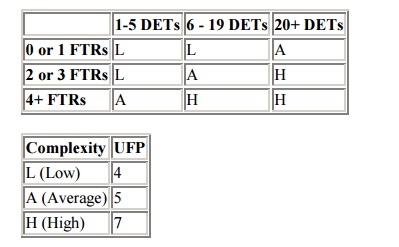
Functional Complexity - The first adjustment factor considers the Functional Complexity for each unique function. Functional Complexity is determined based on the combination of data groupings and data elements of a particular function. The number of data elements and unique groupings are counted and compared to a complexity matrix that will rate the function as low, average or high complexity. Each of the five functional components (ILF, EIF, EI, EO and EQ) has its own unique complexity matrix. The following is the complexity matrix for External Outputs.

Using the examples given above and their appropriate complexity matrices, the function point count for these functions would be:

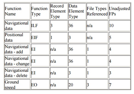
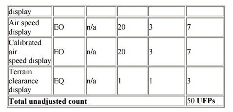
All of the functional components are analyzed in this way and added together to derive an Unadjusted Function Point count.

Value Adjustment Factor - The Unadjusted Function Point count is multiplied by the second adjustment factor called the Value Adjustment Factor. This factor considers the system's technical and operational characteristics and is calculated by answering 14 questions. The factors are:

1. Data Communications

The data and control information used in the application are sent or received over communication facilities.

2. Distributed Data Processing

Distributed data or processing functions are a characteristic of the application within the application boundary.

3. Performance

Application performance objectives, stated or approved by the user, in either response or throughput, influence (or will influence) the design, development, installation and support of the application.

4. Heavily Used Configuration

A heavily used operational configuration, requiring special design considerations, is a characteristic of the application.

5. Transaction Rate

The transaction rate is high and influences the design, development, installation and support.

6. On-line Data Entry

On-line data entry and control information functions are provided in the application.

7. End -User Efficiency

The on-line functions provided emphasize a design for end-user efficiency.

8. On-line Update

The application provides on-line update for the internal logical files.

9. Complex Processing

Complex processing is a characteristic of the application.

10. Reusability

The application and the code in the application have been specifically designed, developed and supported to be usable in other applications.

11. Installation Ease

Conversion and installation ease are characteristics of the application. A conversion and installation plan and/or conversion tools were provided and tested during the system test phase.

12. Operational Ease

Operational ease is a characteristic of the application. Effective start-up, backup and recovery procedures were provided and tested during the system test phase.

13. Multiple Sites

The application has been specifically designed, developed and supported to be installed at multiple sites for multiple organizations.

14. Facilitate Change

The application has been specifically designed, developed and supported to facilitate change.

Each of these factors is scored based on their influence on the system being counted. The resulting score will increase or decrease the Unadjusted Function Point count by 35%. This calculation provides us with the Adjusted Function Point count.

An Approach to Counting Function Points

There are several approaches used to count function points. Q/P Management Group, Inc. has found that a structured workshop conducted with people who are knowledgeable of the functionality provided through the application is an efficient, accurate way of collecting the necessary data. The workshop approach allows the counter to develop a representation of the application from a functional perspective and educate the participants about function points.

Function point counting can be accomplished with minimal documentation. However, the accuracy and efficiency of the counting improves with appropriate documentation. Examples of appropriate documentation are:

·        Design specifications

·        Display designs

·        Data requirements (Internal and External)

·        Description of user interfaces

Function point counts are calculated during the workshop and documented with both a diagram that depicts the application and worksheets that contain the details of each function discussed.

Benefits of Function Point Analysis

Organizations that adopt Function Point Analysis as a software metric realize many benefits including: improved project estimating; understanding project and maintenance productivity; managing changing project requirements; and gathering user requirements. Each of these is discussed below.

Estimating software projects is as much an art as a science. While there are several environmental factors that need to be considered in estimating projects, two key data points are essential. The first is the size of the deliverable. The second addresses how much of the deliverable can be produced within a defined period of time. Size can be derived from Function Points, as described above. The second requirement for estimating is determining how long it takes to produce a function point. This delivery rate can be calculated based on past project performance or by using industry benchmarks. The delivery rate is expressed in function points per hour (FP/Hr) and can be applied to similar proposed projects to estimate effort (i.e. Project Hours = estimated project function points FP/Hr).

Productivity measurement is a natural output of Function Points Analysis. Since function points are technology independent they can be used as a vehicle to compare productivity across dissimilar tools and platforms. More importantly, they can be used to establish a productivity rate (i.e. FP/Hr) for a specific tool set and platform. Once productivity rates are established they can be used for project estimating as described above and tracked over time to determine the impact continuous process improvement initiatives have on productivity.

In addition to delivery productivity, function points can be used to evaluate the support requirements for maintaining systems. In this analysis, productivity is determined by calculating the number of function points one individual can support for a given system in a year (i.e. FP/FTE year). When compared with other systems, these rates help to identify which systems require the most support. The resulting analysis helps an organization develop a maintenance and replacement strategy for those systems that have high maintenance requirements.

Managing Change of Scope for an in-process project is another key benefit of Function Point Analysis. Once a project has been approved and the function point count has been established, it becomes a relatively easy task to identify, track and communicate new and changing requirements. As requests come in from users for new displays or capabilities, function point counts are developed and applied against the rate. This result is then used to determine the impact on budget and effort. The user and the project team can then determine the importance of the request against its impact on budget and schedule. At the conclusion of the project the final function point count can be evaluated against the initial estimate to determine the effectiveness of requirements gathering techniques. This analysis helps to identify opportunities to improve the requirements definition process.

Communicating Functional Requirements was the original objective behind the development of function points. Since it avoids technical terminology and focuses on user requirements it is an excellent vehicle to communicate with users. The techniques can be used to direct customer interviews and document the results of Joint Application Design (JAD) sessions. The resulting documentation provides a framework that describes user and technical requirements.

In conclusion, Function Point Analysis has proven to be an accurate technique for sizing, documenting and communicating a system's capabilities. It has been successfully used to evaluate the functionality of real-time and embedded code systems, such as robot based warehouses and avionics, as well as traditional data processing. As computing environments become increasingly complex, it is proving to be a valuable tool that accurately reflects the systems we deliver and maintain.

COCOMO Model

The COCOMO cost estimation model is used by thousands of software project managers, and is based on a study of hundreds of software projects. Unlike other cost estimation models, COCOMO is an open model, so all of the details are published, including:

·        The underlying cost estimation equations

·        Every assumption made in the model (e.g. "the project will enjoy good management")

·        Every definition (e.g. the precise definition of the Product Design phase of a project)

·        The costs included in an estimate are explicitly stated (e.g. project managers are included, secretaries aren't)

Because COCOMO is well defined, and because it doesn't rely upon proprietary estimation algorithms, Costar offers these advantages to its users:

·        COCOMO estimates are more objective and repeatable than estimates made by methods relying on proprietary models

·        COCOMO can be calibrated to reflect your software development environment, and to produce more accurate estimates

Costar is a faithful implementation of the COCOMO model that is easy to use on small projects, and yet powerful enough to plan and control large projects.

Typically, you'll start with only a rough description of the software system that you'll be developing, and you'll use Costar to give you early estimates about the proper schedule and staffing levels. As you refine your knowledge of the problem, and as you design more of the system, you can use Costar to produce more and more refined estimates.

Costar allows you to define a software structure to meet your needs. Your initial estimate might be made on the basis of a system containing 3,000 lines of code. Your second estimate might be more refined so that you now understand that your system will consist of two subsystems (and you'll have a more accurate idea about how many lines of code will be in each of the subsystems). Your next estimate will continue the process -- you can use Costar to define the components of each subsystem. Costar permits you to continue this process until you arrive at the level of detail that suits your needs.

One word of warning: It is so easy to use Costar to make software cost estimates, that it's possible to misuse it -- every Costar user should spend the time to learn the underlying COCOMO assumptions and definitions from Software Engineering Economics and Software Cost Estimation with COCOMO II.

The most fundamental calculation in the COCOMO model is the use of the Effort Equation to estimate the number of Person-Months required to develop a project. Most of the other COCOMO results, including the estimates for Requirements and Maintenance, are derived from this quantity.

Source Lines of Code

The COCOMO calculations are based on your estimates of a project's size in Source Lines of Code (SLOC). SLOC is defined such that:

·        Only Source lines that are DELIVERED as part of the product are included -- test drivers and other support software is excluded

·        SOURCE lines are created by the project staff -- code created by applications generators is excluded

·        One SLOC is one logical line of code

·        Declarations are counted as SLOC

·        Comments are not counted as SLOC

The original COCOMO 81 model was defined in terms of Delivered Source Instructions, which are very similar to SLOC. The major difference between DSI and SLOC is that a single Source Line of Code may be several physical lines. For example, an "if-then-else" statement would be counted as one SLOC, but might be counted as several DSI.

The Scale Drivers

In the COCOMO II model, some of the most important factors contributing to a project's duration and cost are the Scale Drivers. You set each Scale Driver to describe your project; these Scale Drivers determine the exponent used in the Effort Equation.

The 5 Scale Drivers are:

·        Precedentedness

·        Development Flexibility

·        Architecture / Risk Resolution

·        Team Cohesion

·        Process Maturity

Note that the Scale Drivers have replaced the Development Mode of COCOMO 81. The first two Scale Drivers, Precedentedness and Development Flexibility actually describe much the same influences that the original Development Mode did.

Cost Drivers

COCOMO II has 17 cost drivers � y ou assess your project, development environment, and team to set each cost driver. The cost drivers are multiplicative factors that determine the effort required to complete your software project. For example, if your project will develop software that controls an airplane's flight, you would set the Required Software Reliability (RELY) cost driver to Very High. That rating corresponds to an effort multiplier of 1.26, meaning that your project will require 26% more effort than a typical software project.

.COCOMO II defines each of the cost drivers, and the Effort Multiplier associated with each rating. Check the Costar help for details about the definitions and how to set the cost drivers.

COCOMO II Effort Equation

The COCOMO II model makes its estimates of required effort (measured in Person-Months � PM) based primarily on your estimate of the software project's size (as measured in thousands of SLOC, KSLOC)):

Effort = 2.94 * EAF * (KSLOC)^E

Where

EAF Is the Effort Adjustment Factor derived from the Cost Drivers

E Is an exponent derived from the five Scale Drivers

As an example, a project with all Nominal Cost Drivers and Scale Drivers would have an EAF of 1.00 and exponent, E, of 1.0997. Assuming that the project is projected to consist of 8,000 source lines of code, COCOMO II estimates that 28.9 Person-Months of effort is required to complete it:

Effort = 2.94 * (1.0) * (8)^1.0997 = 28.9 Person-Months

Effort Adjustment Factor

The Effort Adjustment Factor in the effort equation is simply the product of the effort multipliers corresponding to each of the cost drivers for your project.

For example, if your project is rated Very High for Complexity (effort multiplier of 1.34), and Low for Language & Tools Experience (effort multiplier of 1.09), and all of the other cost drivers are rated to be Nominal (effort multiplier of 1.00), the EAF is the product of 1.34 and 1.09.

Effort Adjustment Factor = EAF = 1.34 * 1.09 = 1.46

Effort = 2.94 * (1.46) * (8)^1.0997 = 42.3 Person-Months

COCOMO II Schedule Equation

The COCOMO II schedule equation predicts the number of months required to complete your software project. The duration of a project is based on the effort predicted by the effort equation:

Duration = 3.67 * (Effort)^SE

Where

Effort Is the effort from the COCOMO II effort equation

SE Is the schedule equation exponent derived from the five Scale Drivers

Continuing the example, and substituting the exponent of 0.3179 that is calculated from the scale drivers, yields an estimate of just over a year, and an average staffing of between 3 and 4 people:

Duration = 3.67 * (42.3)^0.3179 = 12.1 months

Average staffing = (42.3 Person-Months) / (12.1 Months) = 3.5 people

The SCED Cost Driver

The COCOMO cost driver for Required Development Schedule (SCED) is unique, and requires a special explanation.

The SCED cost driver is used to account for the observation that a project developed on an accelerated schedule will require more effort than a project developed on its optimum schedule. A SCED rating of Very Low corresponds to an Effort Multiplier of 1.43 (in the COCOMO II.2000 model) and means that you intend to finish your project in 75% of the optimum schedule (as determined by a previous COCOMO estimate). Continuing the example used earlier, but assuming that SCED has a rating of Very Low, COCOMO produces these estimates:

Duration = 75% * 12.1 Months = 9.1 Months

Effort Adjustment Factor = EAF = 1.34 * 1.09 * 1.43 = 2.09

Effort = 2.94 * (2.09) * (8)^1.0997 = 60.4 Person-Months

Average staffing = (60.4 Person-Months) / (9.1 Months) = 6.7 people

Notice that the calculation of duration isn't based directly on the effort (number of Person-Months) � instead it's based on the schedule that would have been required for the project assuming it had been developed on the nominal schedule. Remember that the SCED cost driver means "accelerated from the nominal schedule".

The Costar command Constraints | Constrain Project displays a dialog box that lets you trade off duration vs. effort (SCED is set for you automatically). You can use the dialog box to constrain your project to have a fixed duration, or a fixed cost.