Interpolation And Approximation

INTERPOLATION AND APPROXIMATION

 

1 Interpolation with Unequal Intervals

Lagrange`s Interpolation formula

Inverse Interpolation by Lagrange`s Interpolation Polynomial

2 Divided Differences-Newton Divided Difference Interpolation

Divided Differences

Newtons Divided Difference formula for unequal intervals

3 Interpolating with a cubic spline

Cubic spline interpolation

4 Interpolation with equals

Newtons` forward interpolation formula

Newtons` Backward interpolation formula

 

 

 

1 Interpolation with Unequal intervals

 

Introduction

 

Interpolation is a process of estimating the value of a function at ana intermediate point when its value are known only at certain specified points.It is based on the following assumptions:

 

(i)                Given equation is a polynomial or it can be represented by a polynomial with a good degree of approximation.

 

(ii)             Function should vary in such a way that either it its increasing or decreasing in the given range without sudden jumps or falls of functional values in the given interval.

 

We shall discuss the concept of interpolation from a set of tabulated values of when the values of x are given intervals or at unequal intervals

 

.First we consider interpolation with unequal intervals.

 

 

Lagrange’s Interpolation formula

 

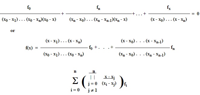
This is called the for Interpolation Lagrange’s. formula

 

Problems

 

1.Using Lagrange’s interpolation find the value of y-corresponding formula, to x=10 from the following data

Using x=10 and the given data, y (10) =14.67

 

 

2. Using Lagrange’s interpolation forfromula,the fi following data

X       3        7        9        10

Y       168    120    72      63

Sol:

 

Given

By Lagrange’s   interpolation   formula

Using x=6 and the given data, y(6)=147

 

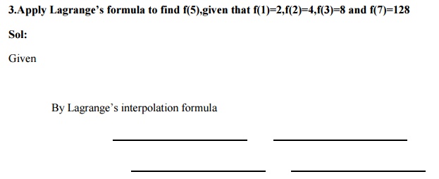
Using x=5 and the given data, y(5)=32.93

 

 

 

Exercise

 

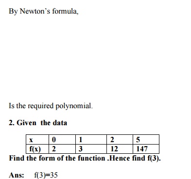
1.Find the polynomial degree 3 fitting the following data

 

X       -1      0        2        3

Y       -2      -1      1        4

Ans:

2.Given

 

Ans:

 

Inverse Interpolation   by   Lagrange’s   interpolating

 

Lagrange’s interpolation formula can be used is not in the table. The process of finding such of x is called inverse interpolation.

 

If x is the dependent variable and y is the independent variable, we can write a formula for x as a function of y.

 

 

 

 

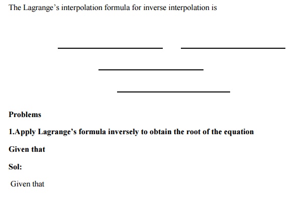
2  Divided Difference –Newton Divided Difference Interpolation Formula

 

Introduction

 

If the values of x are given at unequal intervals, it is convenient to introduce the idea of divided differences. The divided difference are the differences of y=f(x) defined, taking into consideration the changes in the values of the argument .Using divided differences of the function y=f(x),we establish Newton’s which divided is used for different interpolation which the values of x are at unequal intervals and also for fitting an approximate

 

curve for the given data.

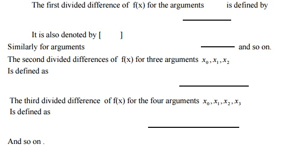
Divided difference

Let the function assume the values Corresponding to the arguments x1 , x2 , x3 ,..... xn respectively, where the intervals  need to be equal.

Definitions

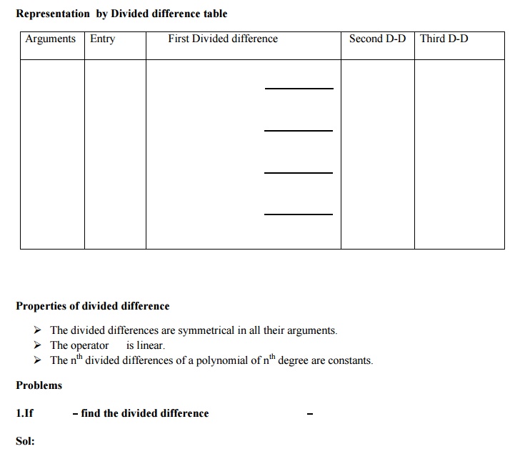
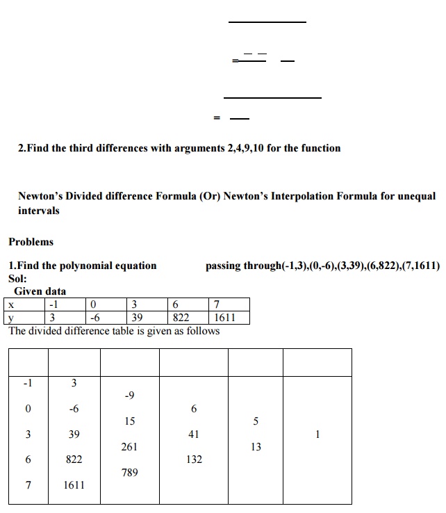
The first divided difference of  f(x) for the arguments is defined by

 

 

 

3 Interpolating with a cubic spline

 

cubic spline Interpolation

 

We consider the problem of interpolation between given data points (x_i, y_i), i=0, 1, 2, 3….n   where  

 by means of a smooth polynomial curve.  

By means of method of least squares, we can fit is the new technique recently developed to fit a smooth curve passing he given set of points.

 

Definition of Cubic spline

 

A cubic spline s(x) is defined by the following properties.

       S(xi)=y_i,i=0,1,2,…..n

       S(x),s’(x),s”(x)   are   continuous   on   [a,b]

       S(x) is a cubic polynomial in each sub-interval(x_i,x_i+1),i=0,1,2,3…..n=1

 

Conditions for fitting spline fit

 

The conditions for a cubic spline fit are that we pass a set of cubic through the points, using a new cubic in each interval. Further it is required both the slope and the curvature be the same for the pair of cubic that join at each point.

Natural cubic spline

A cubic spline s(x) such that s(x) is linear in the intervals 

i.e. s₁=0 and s_n=0 is called a natural cubic spline

 

where       s₁ =second derivative at (x₁ , y₁ )

s_n Second derivative at (x_n , y_n )

Note

 

The three alternative choices used are

with the assumption, for a set of data that are fit by a single cubic equation their cubic splines will all be this same cubic

 

 

Problems

 

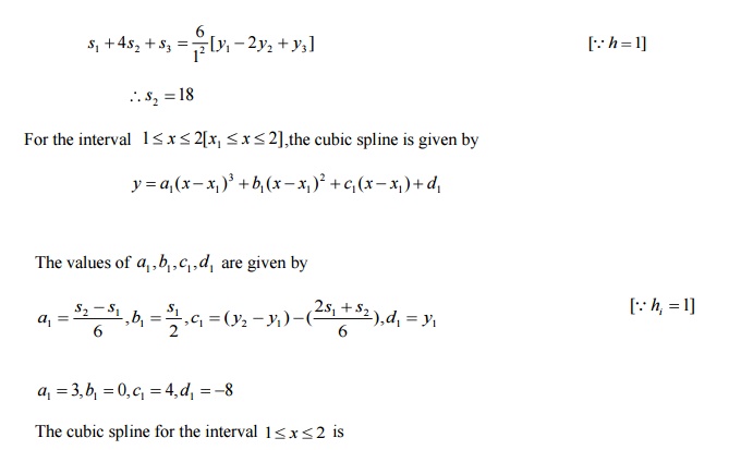
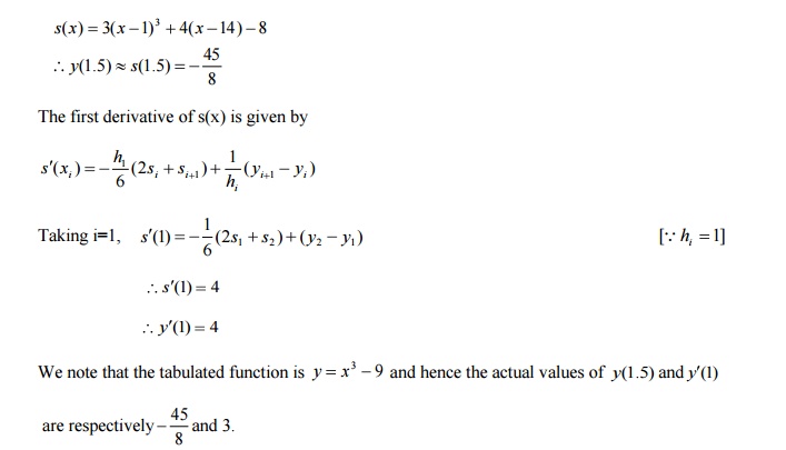
1.Fit a natural cubic spline to the following data

x  1     2     3

y  -8     -1     18

 

And compute (i) y(1.5) (ii) y’(1)

Solution

For equally spaced intervals,the relation on s₁ , s₂  & s₃  is given by

 

 

2.The following values of x and y are given ,obtain the natural cubic spline which agree with y(x) at the set of data points

 

X             2       3        4

Y             11     49      123

 

 

Hence compute (i) y(2.5) and (ii) y’ (2)

Exercise:

 

1.Fit the following data by a cubic spline curve

x              0       1        2                 3        4

y              -8      -7      0                 19      56

Using the end condition that s₁ & s₅  are linear extrapolations.

4 Interpolation with equal intervals

 (Newton’s Forward and Backward Difference formulas)

 Introduction

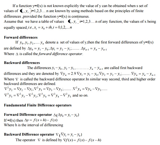
 If a function y=f(x) is not known explicitly the value of y can be obtained when s set of

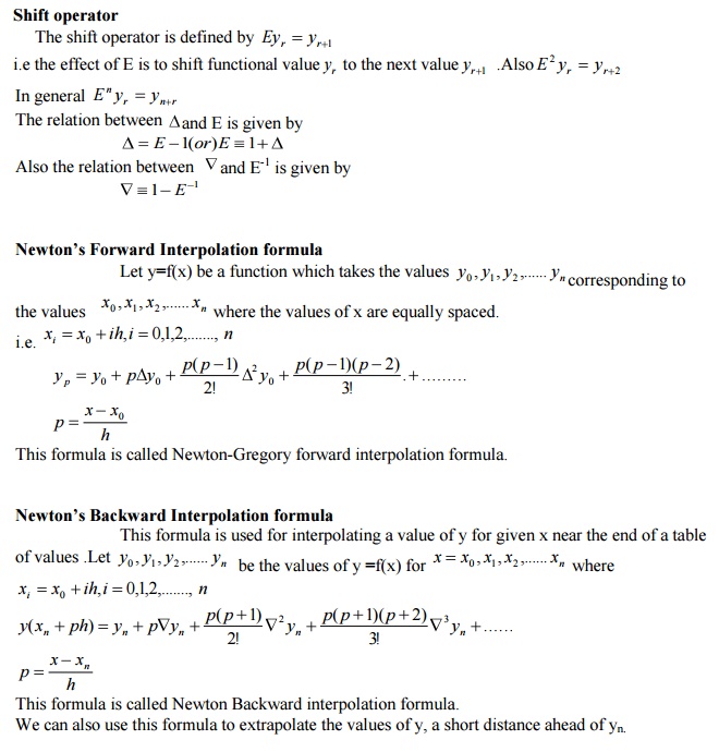
This formula is called Newton Backward interpolation formula.

We can also use this formula to extrapolate the values of y, a short distance ahead of y_n.

 

Problems

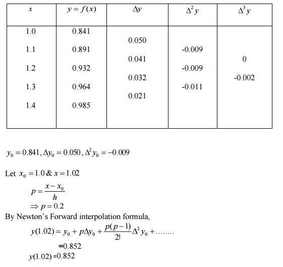
1.Using Newton’s Forward interpolation formula

X      1.0   1.1 1.2 1.3 1.4

F(x)      0.841   0.891 0.932 0.964 0.985

Sol:

Forward difference table:

y(27)=24.8

 

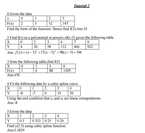
4.Find the cubic polynomial which takes the value y(0)=1,y(1)=0,y(2)=1,y(3)=10.Hence or otherwise ,obtain y(4).Ans:y(4)=33

 

Exercise: 1.Given the data

x        0        1        2        3        4

y        2        3        12      35      78

Find the cubic function of x,using Newton’s backward   interpolation formula

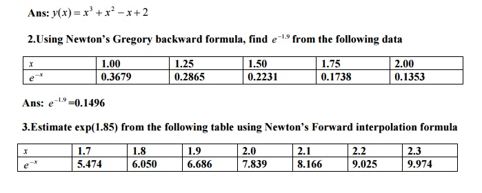
Ans:6.3601

 

4.Find the polynomial which passes through the point newton's   (7,3)(8,1)(9,1)(10,9) using  interpolation formula.

 

 

Tutorial Problems

 

Tutorial 1

 

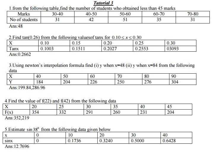
1.Apply Lagrange’s formula inversely to obtai f(0)=-4,f(1)=1,f(3)=29,f(4)=52.

 

Ans: 0.8225

 

2.Using Lagrange’s   formula   of   interpolation   ,

X                       7         8        9        10

Y                       3         1        1        9

Ans: 3.625

 

3.Use Lagrange’s   formula   to   find   the   value   of

x                       3         7        9        10

y                       168     120    72      63

Ans: 147

 

4.If log(300)=2.4771,log(304)=2.4829,log(305)=2.4843,log(307)=2.4871find log(301) Ans: 2.8746

 

 

 

Part A

1.                 State   the   Lagrange’s.   interpolation   formula

 

Sol:

Let y = f(x) be a function which takes the values y₀, y₁,……_n y-corresponding to x=x₀,x₁,……_nx

Then Lagrange’s   interpolation   formula   is

Y = f(x) =  --- --  

 

2.                 What   is   the   assumption   we   make   when   Lagran

Sol:

 

Lagrange’s interpolation formula can be used whether the values of x, the independent variable are equally spaced or not whether the difference of y become smaller or not.

 

3.                 When   Newton’s   backward   interpolation   formu

Sol:

 

The formula is used mainly to interpolate the values of y near the end of a set of tabular values and also for extrapolation the values of y a short distance ahead of y₀

 

4. What are the errors in Trapezoidal rule of numerical integration?

Sol:

The error in the Trapezoidal rule is

E< ---- y”

5.Why   Simpson’s   one   third   rule   is   called   a   c

Sol:

Since the end point ordinates y₀ and y_n are included in the Simpson closed formula.

 

 

6.  What   are   the   advantages   of   Lagrange’sformula?   formul

 

Sol:

 

The forward and backward interpolation formulae of Newton can be used only when the values of theindependent variable x are equally spaced and can also be used when the differences

 

of the dependent variable y become smaller ultimately. But Lagrange’s interpolati be used whether the values of x, the independent variable are equally spaced or not and whether

 

the difference of y become smaller or not.

 

 

7. When   do   we   apply   Lagrange’s   interpolation?

Sol:

 

Lagrange’s formulainterpolcationbe used when the val not. It is mainly used when the values are unevenly spaced.

 

8. When   do   we   apply   Lagrange’s   interpolation?

Sol:

 

Lagrange’s interpolation formula spacedcanor be us not. It is mainly used when the values are unevenly spaced.

 

9.   What   are   the   disadvantages   in   practice   in   ap

Sol:

1. It takes time.

2. It is laborious

 

10.                    When   Newton’s   backwardformulaisused.   interpolation

Sol:

The       formula   is   used   mainly   to   interpolate

 

values.

 

11.                    When   Newton’s   forward   interpolation   formu

Sol:

 

The formula is used mainly tobeginniginterpolateofsetof tabular values.

 

 

12.                    When   do   we   use   Newton’s   divided   differenc

Sol: This is used when the data are unequally spaced.

 

13.  Write Forward difference operator.

 

Sol:

 

Let y = f (x) be a function of x and let of the values of y. corresponding to of the values of x. Here, the independent variable (or argument), x

 

proceeds at equally spaced intervals and h (constant),the difference between two consecutive values of x is called the interval of differencing. Now the forward difference operator is defined as

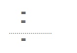
These are called first differences.

 

14.Write Backward difference operator.

Sol:

The backward difference operator is defined as

 

These are called first differences

 

 

 

Part B

 

1.Using   Newton’s   divided   difference and hence formula, find f(4).

X                        0        1        2                 5       

                                                                          

f(x)                      2        3        12               147   

 

 

2.Find the cubic polynomial which takes the following values:

 

X                       0         1        2        3

                                             

f(x)                    1         2        1        10

                                             

3.The following values of x and y are given:

 

X                       1         2        3        4

                                             

f(x)                    1         2        5        11

                                             

Find the cubic splines and evaluate y(1.5) and y’(3).

 

4.Find the rate of growth of the population in 1941 and 1971 from the table below.

Year X              1931   1941  1951  1961  1971

Population        40.62  60.8   79.95 103.56        132.65

Y                                                    

5.Derive            Newton’s   backward   difference   formula

 

6.Using             Lagrange’s   interpolation     formula   fin

 

(0,-12),(1,0),(3,6),(4,12).

7.Using   Newton’s   divided difference   formula

                                                                 

X                       0         1        2        4        5       

f(x)                    1         14      15      5        6       

 

8.Obtain the cubic spline approximation for the function y=f(x) from the following data, given that y0” 3=”=0y.

 

X                       -1        0        1        2

Y                       -1        1        3        35

 

9.The following table gives the values of density of saturated water for various temperatures of saturated steam.

 

Temperature⁰ C 0         100    150    200    250    300   

                                                                          

                                                                          

Density hg/m3    958    917    865    799    712   

Find by interpolation, the density when the temperature is 275⁰ .

 

10.Use Lagrange’s₁₀656 method,giventhatlog ₁₀to654 =2find.8156, log log ₁₀ 658 =2.8182 , log ₁₀ 659 =2.8189 and log ₁₀ 661 =2.8202.

 

11.Find f’(x) at x=1.5 and x=4.0 from the fol differentiation.

 

 

x                       1.5      2.0     2.5     3.0     3.5     4.0

Y=f(x)               3.375  7.0     13.625        24.0   38.875        59.0

 

12.If f(0)=1,f(1)=2,f(2)=33 and f(3)=244. Find a cubic spline approximation, assuming M(0)=M(3)=0.Also find f(2.5).

 

13.Fit a set of 2 cubic splines to a half ellipse described by f(x)= [25-4x²]^1/2. Choose the three data points (n=2) as (-2.5,0), (0,1.67) and (2.5 , 0) and use the free boundary conditions.

 

14.Find the value of y at x=21 and x=28 from the data given below

 

x                       20       23      26      29

y                       0.3420 0.3907        0.4384        0.4848

15. The population of a town is as follows:

 

x year                1941   1951  1961  1971           1981  1991

                                                                          

y population     20       24      29      36               46      51

(thousands)                                                        

                                                                          

Estimate the population increase during the period 1946 to1976.