Ideal and Real Gases, Thermodynamic Relations

IDEAL AND REAL GASES, THERMODYNAMIC RELATIONS

IDEAL GAS

An ideal gas is a theoretical gas composed of a set of randomly-moving point particles that interact only through elastic collisions. The ideal gas concept is useful because it obeys the ideal gas law, a simplified equation of state, and is amenable to analysis under statistical mechanics.

At normal ambient conditions such as standard temperature and pressure, most real gases behave qualitatively like an ideal gas. Generally, deviation from an ideal gas tends to decrease with higher temperature and lower density, as the work performed by intermolecular forces becomes less significant compared with the particles' kinetic energy, and the size of the molecules becomes less significant compared to the empty space between them.

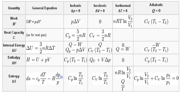
EQUATION TABLE FOR AN IDEAL GAS

REAL GAS

Real gas, as opposed to a Perfect or Ideal Gas, effects refers to an assumption base where the following are taken into account:

•Compressibility effects

•Variable heat capacity

•Van der Waals forces

•Non-equilibrium thermodynamic effects

•Issues with molecular dissociation and elementary reactions with variable composition.

For most applications, such a detailed analysis is "over-kill" and the ideal gas approximation is used. Real-gas models have to be used near condensation point of gases, near critical point, at very high pressures, and in several other less usual cases.

VAN DER WAALS MODELISATION

Real gases are often modeled by taking into account their molar weight and molar volume

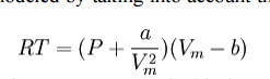
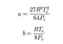
Where P is the pressure, T is the temperature, R the ideal gas constant, and Vm the molar volume. a and b are parameters that are determined empirically for each gas, but are sometimes estimated from their critical temperature (Tc) and critical pressure (Pc) using these relations:

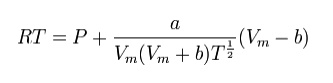
REDLICH–KWONG MODELISATION

The Redlich–Kwong equation is another two-parameters equation that is used to modelize real gases. It is almost always more accurate than the Van der Waals equation, and often more accurate than some equation with more than two parameters. The equation is

THERMODYNAMICS RELATIONS

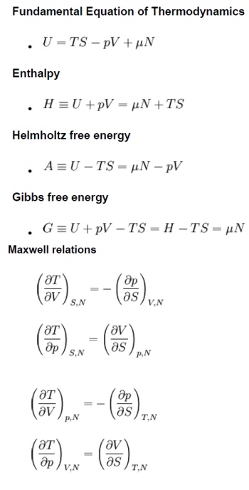
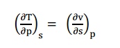
Maxwell     relations.

The Maxwell’s equations relate entro properties p,v and T for pure simple compressible substances.

From first law of thermodynamics,                                        

Q = W +  U                                                

Rearranging the parameters                                                   

Q =  U + W since [ds =            , W = pdv ]

Tds = du +pdv                                                    

du = Tds –pdv     ----------- (1)                   

We know that, h = u + pv                                                      

dh = du + d(pv)                                                   

= du + vdp + pdv          ----------- (2)

Substituting the value du in equation (2),           

dh = Tds + pdv + vdp –pdv                                         

dh = Tds + vdp    ----------- (3)                   

By   Helmotz’s   function,      

a = u –Ts                                                   

da = du –d(Ts)                                                    

= du –Tds –sdT             ----------- (4)

Substituting the values of du in equation (4),               

da = Tds –pdv –Tds –sdT                                            

T = –pdv –sdT     ----------- (5)                   

By Gibbs functions,                                                      

G = h –Ts                                                  

dg = dh –d(Ts)                                                    

dg = dh –Tds –sdT        ----------- (6)

Substituting the value of dh in equation (6),

So, dg becomes

dg = Tds + vdp –Tds –sdT

dg = vdp –sdT      ----------- (7)

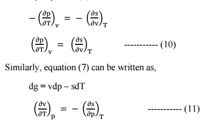
By inverse exact differential we can write equation (1) as, du = Tds –pdv

----------- (8)

Similarly, equation (3) can be written as, dh = Tds + vdp

----------- (9)

Similarly, equation (5) can be written as,

These equations 8, 9,   10   and   11   are   Maxwell’s   e

Tds relations in terms of temperature and pressure changes and temperature and volume changes.

The entropy (s) of pure substance can be expressed as a function of temperature (T) and pressure (p).

s = f(T,p)

We know that,

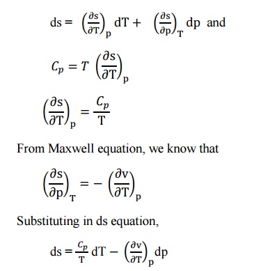
This is known as the first form of entropy equation or the first Tds equation. By considering the entropy of a pure substance as a function of temperature and specific volume,

i.e.    s = f(T,v)

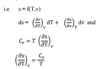
From the Maxwell Equations, we know that

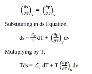
This is known as the second form of entropy equation or the second Tds equation

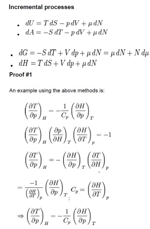
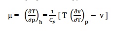
THE JOULE-THOMSON COEFFICIENT OF AN IDEAL GAS IS ZERO

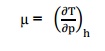
The Joule-Thomson coefficient is defined as the change in temperature with change in pressure, keeping the enthalpy remains constant. It is denoted by,

We know that the equation of state as,

pV=RT

Differentiating the above equation of state with respect to T by keeping pressure, p constant.

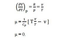
It implies that the Joule-Thomson coefficient is zero for ideal gas.

CLAUSIUS–CLAPEYRON RELATION

The Clausius–Clapeyron relation, named after Rudolf Clausius and Émile Clapeyron, who defined it sometime after 1834, is a way of characterizing the phase transition between two phases of matter, such as solid and liquid. On a pressure–temperature (P–T) diagram, the line separating the two phases is known as the coexistence curve. The Clausius–Clapeyron relation gives the slope of this curve. Mathematically,

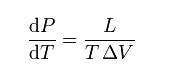
where dP / dT is the slope of the coexistence curve, L is the latent heat, T is the temperature,Visthevolumeandchange of the phase transition.

Pressure Temperature Relations

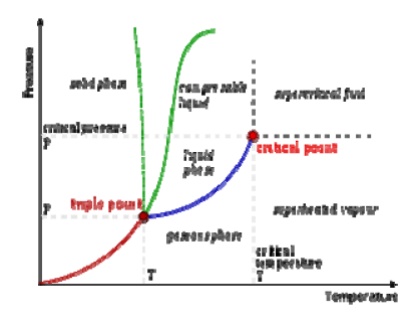
A typical phase diagram. The dotted line gives the anomalous behavior of water. The Clausius–Clapeyron relation can be used to (numerically) find the relationships between pressure and temperature for the phase change boundaries. Entropy and volume changes (due to phase change) are orthogonal to the plane of this drawing

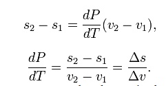
Derivation

Using the state postulate, take the specific entropy, s, for a homogeneous substance to be a function of specific volume, v, and temperature, T.

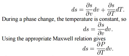
Since temperature and pressure are constant during a phase change, the derivative of pressure with respect to temperature is not a function of the specific volume. Thus the partial derivative may be changed into a total derivative and be factored out when taking an integral from one phase to another,

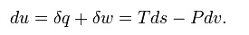
Del is used as an operator to represent— final (2) minus initial (1) For a closed system undergoing an internally reversible process, the first law is

This leads to a version of the Clausius–Clapeyron equation that is simpler to integrate:

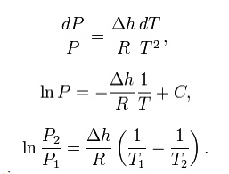
C is a constant of integration

These last equations are useful because they relate saturation pressure and saturation temperature to the enthalpy of phase change, without requiring specific volume data. Note that in this last equation, the subscripts 1 and 2 correspond to different locations on the pressure versus temperature phase lines. In earlier equations, they corresponded to different specific volumes and entropies at the same saturation pressure and temperature.

The Joule–Thomson (Kelvin) coefficient

The rate of change of temperature T with respect to pressure P in a Joule– Thomson process (that is, at constant enthalpy H) is the Joule–Thomson (Kelvin) coefficient μJT. Thisin termscoefficientofthegas'svolumeV, can

its heat capacity at constant pressure Cp, a as

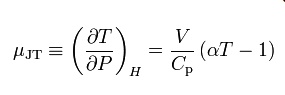
See the Appendix for the proof of thi expressed in °C/bar (SI units: K/Pa) and depends on the type of gas and on the temperature and pressure of the gas before expansion.

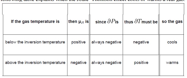
All real gases have an inversion point at which the value of sign. The temperature of this point, the Joule–Thomson inversion temperature,

depends on the pressure of the gas before expansion. In a gas expansion the pressure decreases, so the sign of is always negative. With that in mind, the following table explains when the Joule–Thomson effect cools or warms a real gas:

Helium and hydrogen are two gases whose Joule–Thomson inversion temperatures

at a pressure of one atmosphere forare v helium). Thus, helium and hydrogen warm up when expanded at constant enthalpy

at typical room temperatures. On the other hand nitrogen and oxygen, the two most abundant gases in air, have inversion temperatures of 621 K (348 °C) and 764 K (491 °C) respectively: these gases can be cooled from room temperature by the Joule–Thomson effect.

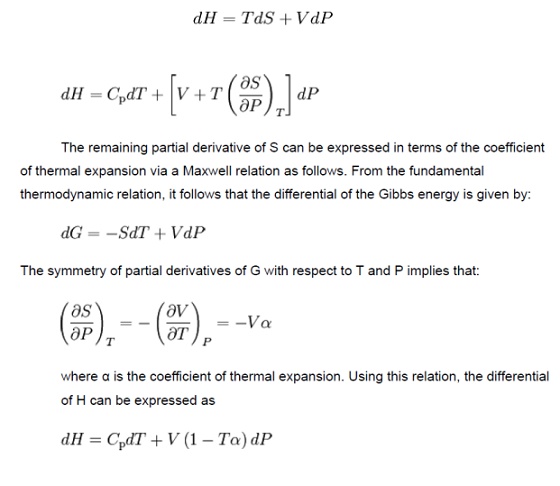
Derivation of the Joule–Thomson (Kelvin) coefficent

A derivation of the formula

for the Joule–Thomson (Kelvin) coefficient.

The partial derivative of T with respect to P at constant H can be computed by expressing the differential of the enthalpy dH in terms of dT and dP, and equating the resulting expression to zero and solving for the ratio of dT and dP. It follows from the fundamental thermodynamic relation that the differential of the enthalpy is given by:

SOLVED PROBLEMS

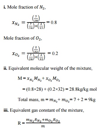
1.       A mixture of ideal gases consists of 7kg ofand 2kg ofat a pressure of 4bar    and a temperature of 27°C. Determine:

i.           Mole fraction of each constituent,

ii.           Equivalent molecular weight of the mixture,

iii.           Equivalent gas constant of the mixture,

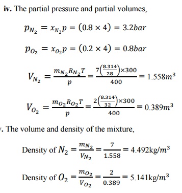
iv.          The partial pressure and partial volumes,

v.           The volume and density of the mixture

Given data:

= 7kg

= 2kg p = 4bar T = 27°C

Solution:

i. Mole fraction of    ,

Describe Joule Kelvin effect with the help of T-p diagram

The Joule Kelvin effect or Joule Thomson effect is an efficient way of cooling gases. In this, a gas is made to undergo a continuous throttling process. A constant pressure is maintained at one side of a porous plug and a constant lower pressure at the other side. The apparatus is thermally insulated so that the heat loss can be measured.

Joule –Thomson co –efficient is defined as the change in temperature with change in pressure, keeping the enthalpy remains constant. It is denoted by,

Throttling process:

It is defined as the fluid expansion through a minute orifice or slightly opened valve. During this process, pressure and velocity are reduced. But there is no heat transfer and no work done by the system. In this process enthalpy remains constant.

Joule Thomson Experiment:

The figure shows the arrangement of porous plug experiment. In this experiment, a stream of gas at a pressure and temperature is allowed to flow continuously through a porous pig. The gas comes out from the other side of the porous pig at a pressure and temperature .

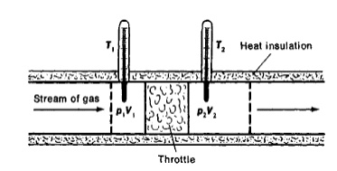
The whole apparatus is insulated. Therefore no heat transfer takes place. Q = 0.

The system does not exchange work with the surroundings.

So, W=0 from steady flow energy equation we know that

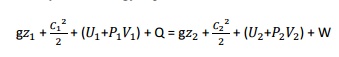
Since there is no considerable change velocity,  and , Q=0,W=0, are applied in steady  flow energy equation. Therefore, It indicates that the enthalpy is constant for throttling process.

It is assumed that a series of experiments performed on a real gas keeping the initial pressure p1 and temperature T1 constant with various down steam pressures ( p2,p3..... ). It is found that the down steam temperature also changes. The results from these experiments can be plotted as enthalpy curve on T-p plane.

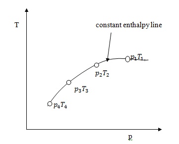
The slope of a constant enthalpy is known as Joule Thomson Coefficient. It is denoted by µ.

For real gas, µ may be either positive or negative depending upon the thermodynamic state of the gas.

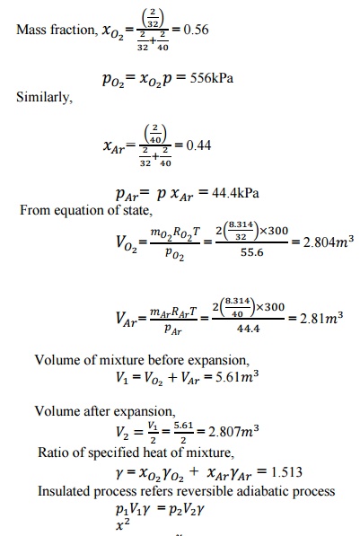
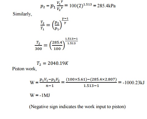
2.     A mixture of 2kg oxygen and 2kg Argon is in an insulated piston cylinder arrangement at 100kPa, 300K. The piston now compresses the mixture to half its initial volume. Molecular weight of oxygen is 40. Ratio of specific heats for oxygen is 1.39 and for argon is 1.667.

Given data:

=2kg =2kg

= 100kPa

= 300K

= 32 = 40

=       =1.39 =1.667