Chapter: Modern Analytical Chemistry: Kinetic Methods of Analysis
Flow Injection Analysis: Theory and Practice
Theory and Practice
Flow injection analysis (FIA) was
developed in the
mid-1970s as a highly efficient technique for
the automated analyses of samples.
Unlike the centrifugal analyzer described earlier, in which samples
are simultaneously analyzed
in batches of limited
size, FIA allows for the rapid, sequential analysis of an unlimited
number of samples. FIA is one member
of a class of techniques called continuous-
flow analyzers, in which samples are introduced sequentially at regular
intervals into a liquid
carrier stream that
transports the samples
to the detector.
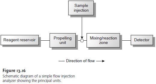
Figure 13.16 is a schematic diagram detailing the basic components of a flow injection analyzer. The reagent serving as the carrier is stored in a reservoir, and a propelling unit maintains a constant flow of the carrier through the system of tub- ing comprising the instrument. The sample is injected directly into the flowing car- rier stream, where it travels through a mixing and reaction zone before passing through the detector’s flow-cell. Figure 13.16 is the simplest design for a flow injec- tion analyzer, consisting of a single channel with one reagent reservoir. Multiple- channel instruments, in which reagents contained in separate reservoirs are combined by merging channels, also are possible. A more detailed discussion of FIA instru- mentation is found in the next section.
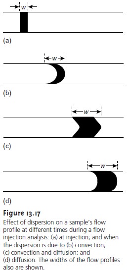
When a sample
is injected into
the carrier stream
it has the
rectangular flow profile (of
width w) shown in Figure 13.17a.
As the sample
is carried through
the mixing and reaction
zone, the width of the flow profile
increases as the sample dis- perses into the carrier stream.
Dispersion results from two processes: convection
due to the flow of the carrier
stream and diffusion due to a concentration gradient between the sample and
the carrier stream.
Convection of the
sample occurs by laminar flow, in which
the linear velocity of the sample
at the tube’s
walls is zero, while the sample at the center
of the tube moves with a linear
velocity twice that of
the carrier stream. The result
is the parabolic flow profile
shown in Figure
13.7b. Convection is the primary means
of dispersion in the first
100 ms following the
sample’s injection.
The second contribution to the sample’s
dispersion is diffusion due to the con-
centration gradient between the sample and the carrier stream. Diffusion occurs
parallel (axial) and perpendicular (radial)
to the flow of the carrier stream,
with only the latter
contribution being important. Radial diffusion decreases the linear velocity of the sample
at the center of the tubing, but the sample
at the edge of the tubing experiences an increase
in its linear velocity. Diffusion helps to maintain
the integrity of the sample’s flow profile (Figure
13.17c), preventing samples
in the car- rier stream from dispersing into one another.
Both convection and diffusion make significant contributions to dispersion from approximately 3–20 s after
the sample’s injection. This
is the normal
time scale for
a flow injection analysis. After approxi- mately 25 s, diffusion becomes the only
significant contributor to dispersion, result- ing in a flow
profile similar to that shown
in Figure 13.17d.
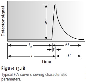
An FIA curve,
or “fiagram,” is a plot of the detector’s signal as a function of time. Figure 13.18 shows a typical
fiagram for conditions in which both convection
and diffusion contribute to the sample’s dispersion. Also shown
on the figure
are several parameters used to characterize the fiagram. Two parameters are used to de-
fine the time required for the sample
to move from the injector
to the detector. The travel time,
ta, is the elapsed
time from the sample’s injection to the arrival
of the leading edge of its flow profile
at the detector. Residence time, T, on the other hand, is
the time required
to obtain the maximum signal.
The difference between
the resi- dence time and travel time is given as t’. The value for t’ approaches 0 when convec- tion is the primary
means of dispersion and increases in value as the contribution from diffusion becomes more important.
The time required
for the sample
to pass through
the detector’s flow cell,
and for the signal to return to the baseline, is also described by two parame- ters. The baseline-to-baseline time,
∆t, is the elapsed
time between the arrival
of the leading edge of the sample’s flow profile to the departure of its trailing edge. The elapsed time
between the maximum
signal and its
return to the baseline is called the return time,
T
‘. The final
characteristic parameter of a fi- agram is the peak height, h, which
is equivalent to the difference between the maximum signal and the signal at the baseline.
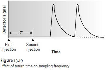
Of the six parameters shown in Figure 13.18, the most important are peak height and return time. The peak height is related, directly or indirectly, to the analyte’s concentration and is used for quantitative work. The sensitiv- ity of the method, therefore, is also determined by the peak height. The return time determines the frequency with which samples may be injected. Figure 13.19 shows that when a second sample is injected at a time T ‘ after injecting the first sample, the overlap of the two FIA curves is minimal. By injecting samples at intervals of T ‘, the maximum sampling rate is realized.
Peak heights and return times are influenced by the dispersion of the sample’s flow profile and are
influenced by the
physical and chemical properties of the
flow injection system. Physical
parameters affecting the peak height
and return time in-
clude the volume of sample injected; the flow rate; the length,
diameter, and geom- etry of the mixing
and reaction zone;
and the presence
of mixing points
where sep- arate channels
merge together. The kinetics of any chemical
reactions involving the sample and reagents in the carrier
stream also influences the peak height and re- turn
time.
Unfortunately, there is no good theory that can be used to consistently predict the peak height and
return time for
a given set
of physical and
chemical parameters. The design
of a flow injection analyzer
for a particular analytical problem
still oc- curs largely
by a process of experimentation. Nevertheless, some general
observa- tions about the effects of physical and chemical parameters can be made.
In the ab- sence of chemical
effects, sensitivity (larger
peak height) is improved by injecting
larger samples, increasing the flow rate, decreasing the length and diameter of the
tubing in the mixing and reaction zone,
and merging separate
channels before the point where the sample
is injected. Except
for sample volume,
an improvement in the
sampling rate (smaller
return time) is achieved by the same combination of physical parameters. Larger sample
volumes, however, lead to longer
return times and a decrease in sample throughput. The effect of chemical reactivity depends on whether the species monitored
by the detector is a reactant or a product.
For exam- ple, when the monitored species is a reactant, sensitivity is improved by selecting a combination of physical parameters that enables the sample to reach the detector
more quickly. Adjusting the chemical
composition of the carrier stream
in a man- ner that decreases the rate of the reaction also improves sensitivity in this case.
Related Topics