Basic Retrieval Queries in SQL

Basic Retrieval Queries in SQL

SQL has one basic statement for retrieving information from a database: the SELECT statement. The SELECT statement is not the same as the SELECT operation of relational algebra, which we discuss in Chapter 6. There are many options and flavors to the SELECT statement in SQL, so we will introduce its features gradually. We will use sample queries specified on the schema of Figure 3.5 and will refer to the sample database state shown in Figure 3.6 to show the results of some of the sample queries. In this section, we present the features of SQL for simple retrieval queries. Features of SQL for specifying more complex retrieval queries are presented in Section 5.1.

Before proceeding, we must point out an important distinction between SQL and the formal relational model discussed in Chapter 3: SQL allows a table (relation) to have two or more tuples that are identical in all their attribute values. Hence, in gen-eral, an SQL table is not a set of tuples, because a set does not allow two identical members; rather, it is a multiset (sometimes called a bag) of tuples. Some SQL rela-tions are constrained to be sets because a key constraint has been declared or because the DISTINCT option has been used with the SELECT statement (described later in this section). We should be aware of this distinction as we discuss the examples.

1. The SELECT-FROM-WHERE Structure of Basic SQL Queries

                     Queries in SQL can be very complex. We will start with simple queries, and then progress to more complex ones in a step-by-step manner. The basic form of the SELECT statement, sometimes called a mapping or a select-from-where block, is formed of the three clauses SELECT, FROM, and WHERE and has the following form:

SELECT <attribute list>

FROM <table list>

WHERE <condition>;

where

                                                    <attribute list> is a list of attribute names whose values are to be retrieved by the query.

                                                    <table list> is a list of the relation names required to process the query.

                                                    <condition> is a conditional (Boolean) expression that identifies the tuples to be retrieved by the query.

In SQL, the basic logical comparison operators for comparing attribute values with one another and with literal constants are =, <, <=, >, >=, and <>. These correspond to the relational algebra operators =, <, ≤, >, ≥, and ≠, respectively, and to the C/C++ programming language operators =, <, <=, >, >=, and !=. The main syntactic difference is the not equal operator. SQL has additional comparison operators that we will present gradually.

We illustrate the basic SELECT statement in SQL with some sample queries. The queries are labeled here with the same query numbers used in Chapter 6 for easy cross-reference.

Query 0. Retrieve the birth date and address of the employee(s) whose name is ‘John B. Smith’.

Q0: SELECT Bdate, Address

FROM EMPLOYEE

WHERE Fname=‘John’ AND Minit=‘B’ AND Lname=‘Smith’;

This query involves only the EMPLOYEE relation listed in the FROM clause. The query selects the individual EMPLOYEE tuples that satisfy the condition of the WHERE clause, then projects the result on the Bdate and Address attributes listed in the SELECT clause.

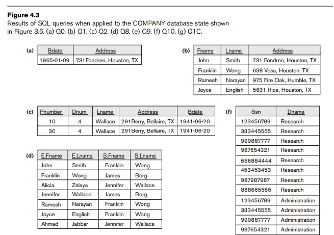
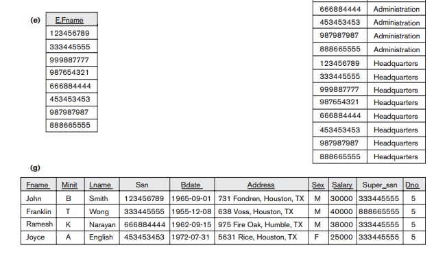
The SELECT clause of SQL specifies the attributes whose values are to be retrieved, which are called the projection attributes, and the WHERE clause specifies the Boolean condition that must be true for any retrieved tuple, which is known as the selection condition. Figure 4.3(a) shows the result of query Q0 on the database of Figure 3.6.

We can think of an implicit tuple variable or iterator in the SQL query ranging or looping over each individual tuple in the EMPLOYEE table and evaluating the condition in the WHERE clause. Only those tuples that satisfy the condition—that is,

those tuples for which the condition evaluates to TRUE after substituting their cor-responding attribute values—are selected.

Query 1. Retrieve the name and address of all employees who work for the ‘Research’ department.

Q1: SELECT Fname, Lname, Address

 FROM EMPLOYEE, DEPARTMENT

 WHERE Dname=‘Research’ AND Dnumber=Dno;

In the WHERE clause of Q1, the condition Dname = ‘Research’ is a selection condi-tion that chooses the particular tuple of interest in the DEPARTMENT table, because Dname is an attribute of DEPARTMENT. The condition Dnumber = Dno is called a join condition, because it combines two tuples: one from DEPARTMENT and one from EMPLOYEE, whenever the value of Dnumber in DEPARTMENT is equal to the value of Dno in EMPLOYEE. The result of query Q1 is shown in Figure 4.3(b). In general, any number of selection and join conditions may be specified in a single SQL query.

A query that involves only selection and join conditions plus projection attributes is known as a select-project-join query. The next example is a select-project-join query with two join conditions.

Query 2. For every project located in ‘Stafford’, list the project number, the controlling department number, and the department manager’s last name, address, and birth date.

Q2: SELECT Pnumber, Dnum, Lname, Address, Bdate

 FROM PROJECT, DEPARTMENT, EMPLOYEE

 WHERE Dnum=Dnumber AND Mgr_ssn=Ssn AND

  Plocation=‘Stafford’;

The join condition Dnum = Dnumber relates a project tuple to its controlling department tuple, whereas the join condition Mgr_ssn = Ssn relates the controlling department tuple to the employee tuple who manages that department. Each tuple in the result will be a combination of one project, one department, and one employee that satisfies the join conditions. The projection attributes are used to choose the attributes to be displayed from each combined tuple. The result of query Q2 is shown in Figure 4.3(c).

2. Ambiguous Attribute Names, Aliasing, Renaming, and Tuple Variables

In SQL, the same name can be used for two (or more) attributes as long as the attributes are in different relations. If this is the case, and a multitable query refers to two or more attributes with the same name, we must qualify the attribute name with the relation name to prevent ambiguity. This is done by prefixing the relation name to the attribute name and separating the two by a period. To illustrate this, suppose that in Figures 3.5 and 3.6 the Dno and Lname attributes of the EMPLOYEE relation were called Dnumber and Name, and the Dname attribute of DEPARTMENT was also called Name; then, to prevent ambiguity, query Q1 would be rephrased as shown in Q1A. We must prefix the attributes Name and Dnumber in Q1A to specify which ones we are referring to, because the same attribute names are used in both relations:

Q1A: SELECT Fname, EMPLOYEE.Name, Address

FROM EMPLOYEE, DEPARTMENT

WHERE DEPARTMENT.Name=‘Research’ AND

DEPARTMENT.Dnumber=EMPLOYEE.Dnumber;

Fully qualified attribute names can be used for clarity even if there is no ambiguity in attribute names. Q1 is shown in this manner as is Q1 below. We can also create an alias for each table name to avoid repeated typing of long table names (see Q8 below).

Q1 : SELECT EMPLOYEE.Fname, EMPLOYEE.LName,

EMPLOYEE.Address

FROM EMPLOYEE, DEPARTMENT

WHERE DEPARTMENT.DName=‘Research’ AND

DEPARTMENT.Dnumber=EMPLOYEE.Dno;

The ambiguity of attribute names also arises in the case of queries that refer to the same relation twice, as in the following example.

Query 8. For each employee, retrieve the employee’s first and last name and the first and last name of his or her immediate supervisor.

Q8: SELECT E.Fname, E.Lname, S.Fname, S.Lname

 FROM EMPLOYEE AS E, EMPLOYEE AS S

 WHERE E.Super_ssn=S.Ssn;

In this case, we are required to declare alternative relation names E and S, called aliases or tuple variables, for the EMPLOYEE relation. An alias can follow the key-word AS, as shown in Q8, or it can directly follow the relation name—for example, by writing EMPLOYEE E, EMPLOYEE S in the FROM clause of Q8. It is also possible to rename the relation attributes within the query in SQL by giving them aliases. For example, if we write

EMPLOYEE AS E(Fn, Mi, Ln, Ssn, Bd, Addr, Sex, Sal, Sssn, Dno)

in the FROM clause, Fn becomes an alias for Fname, Mi for Minit, Ln for Lname, and so on.

In Q8, we can think of E and S as two different copies of the EMPLOYEE relation; the first, E, represents employees in the role of supervisees or subordinates; the second, S, represents employees in the role of supervisors. We can now join the two copies. Of course, in reality there is only one EMPLOYEE relation, and the join condition is meant to join the relation with itself by matching the tuples that satisfy the join con-dition E.Super_ssn = S.Ssn. Notice that this is an example of a one-level recursive query, as we will discuss in Section 6.4.2. In earlier versions of SQL, it was not pos-sible to specify a general recursive query, with an unknown number of levels, in a single SQL statement. A construct for specifying recursive queries has been incorpo-rated into SQL:1999 (see Chapter 5).

The result of query Q8 is shown in Figure 4.3(d). Whenever one or more aliases are given to a relation, we can use these names to represent different references to that same relation. This permits multiple references to the same relation within a query.

We can use this alias-naming mechanism in any SQL query to specify tuple vari-ables for every table in the WHERE clause, whether or not the same relation needs to be referenced more than once. In fact, this practice is recommended since it results in queries that are easier to comprehend. For example, we could specify query Q1 as in Q1B:

Q1B: SELECT E.Fname, E.LName, E.Address

FROM EMPLOYEE E, DEPARTMENT D

WHERE D.DName=‘Research’ AND D.Dnumber=E.Dno;

2. Unspecified WHERE Clause and Use of the Asterisk

We discuss two more features of SQL here. A missing WHERE clause indicates no condition on tuple selection; hence, all tuples of the relation specified in the FROM clause qualify and are selected for the query result. If more than one relation is specified in the FROM clause and there is no WHERE clause, then the CROSS PRODUCT—all possible tuple combinations—of these relations is selected. For example, Query 9 selects all EMPLOYEE Ssns (Figure 4.3(e)), and Query 10 selects all combinations of an EMPLOYEE Ssn and a DEPARTMENT Dname, regardless of whether the employee works for the department or not (Figure 4.3(f)).

Queries 9 and 10. Select all EMPLOYEE Ssns (Q9) and all combinations of

EMPLOYEE Ssn and DEPARTMENT Dname (Q10) in the database.

Q9: SELECT Ssn

 FROM EMPLOYEE;

Q10: SELECT Ssn, Dname

 FROM EMPLOYEE, DEPARTMENT;

It is extremely important to specify every selection and join condition in the WHERE clause; if any such condition is overlooked, incorrect and very large relations may result. Notice that Q10 is similar to a CROSS PRODUCT operation fol-lowed by a PROJECT operation in relational algebra (see Chapter 6). If we specify all the attributes of EMPLOYEE and DEPARTMENT in Q10, we get the actual CROSS PRODUCT (except for duplicate elimination, if any).

To retrieve all the attribute values of the selected tuples, we do not have to list the attribute names explicitly in SQL; we just specify an asterisk (*), which stands for all the attributes. For example, query Q1C retrieves all the attribute values of any EMPLOYEE who works in DEPARTMENT number 5 (Figure 4.3(g)), query Q1D retrieves all the attributes of an EMPLOYEE and the attributes of the DEPARTMENT in which he or she works for every employee of the ‘Research’ department, and Q10A specifies the CROSS PRODUCT of the EMPLOYEE and DEPARTMENT relations.

Q1C: SELECT *

 FROM EMPLOYEE

 WHERE Dno=5;

Q1D: SELECT *

 FROM EMPLOYEE, DEPARTMENT

 WHERE Dname=‘Research’ AND Dno=Dnumber;

Q10A: SELECT *

          FROM        EMPLOYEE, DEPARTMENT;

4. Tables as Sets in SQL

As we mentioned earlier, SQL usually treats a table not as a set but rather as a multiset; duplicate tuples can appear more than once in a table, and in the result of a query. SQL does not automatically eliminate duplicate tuples in the results of queries, for the following reasons:

              Duplicate elimination is an expensive operation. One way to implement it is to sort the tuples first and then eliminate duplicates.

              The user may want to see duplicate tuples in the result of a query.

              When an aggregate function (see Section 5.1.7) is applied to tuples, in most cases we do not want to eliminate duplicates.

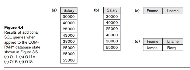
An SQL table with a key is restricted to being a set, since the key value must be distinct in each tuple. If we do want to eliminate duplicate tuples from the result of an SQL query, we use the keyword DISTINCT in the SELECT clause, meaning that only distinct tuples should remain in the result. In general, a query with SELECT DISTINCT eliminates duplicates, whereas a query with SELECT ALL does not. Specifying SELECT with neither ALL nor DISTINCT—as in our previous examples— is equivalent to SELECT ALL. For example, Q11 retrieves the salary of every employee; if several employees have the same salary, that salary value will appear as many times in the result of the query, as shown in Figure 4.4(a). If we are interested only in distinct salary values, we want each value to appear only once, regardless of how many employees earn that salary. By using the keyword DISTINCT as in Q11A, we accomplish this, as shown in Figure 4.4(b).

Query 11. Retrieve the salary of every employee (Q11) and all distinct salary values (Q11A).

Q11:  SELECT     ALL Salary

          FROM        EMPLOYEE;

Q11A:         SELECT     DISTINCT Salary

          FROM        EMPLOYEE;

SQL has directly incorporated some of the set operations from mathematical set theory, which are also part of relational algebra (see Chapter 6). There are set union (UNION), set difference (EXCEPT), and set intersection (INTERSECT) operations. The relations resulting from these set operations are sets of tuples; that is, duplicate tuples are eliminated from the result. These set operations apply only to union-com-patible relations, so we must make sure that the two relations on which we apply the operation have the same attributes and that the attributes appear in the same order in both relations. The next example illustrates the use of UNION.

Query 4. Make a list of all project numbers for projects that involve an employee whose last name is ‘Smith’, either as a worker or as a manager of the department that controls the project.

Q4A:                             ( SELECT DISTINCT Pnumber

FROM                                          PROJECT, DEPARTMENT, EMPLOYEE

WHERE                                        Dnum=Dnumber AND Mgr_ssn=Ssn

AND Lname=‘Smith’ )

UNION

( SELECT                                     DISTINCT Pnumber

FROM                                          PROJECT, WORKS_ON, EMPLOYEE

WHERE                                        Pnumber=Pno AND Essn=Ssn

AND Lname=‘Smith’ );

The first SELECT query retrieves the projects that involve a ‘Smith’ as manager of the department that controls the project, and the second retrieves the projects that involve a ‘Smith’ as a worker on the project. Notice that if several employees have the last name ‘Smith’, the project names involving any of them will be retrieved. Applying the UNION operation to the two SELECT queries gives the desired result.

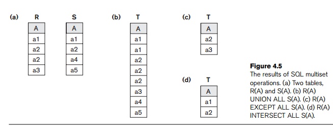
SQL also has corresponding multiset operations, which are followed by the keyword ALL (UNION ALL, EXCEPT ALL, INTERSECT ALL). Their results are multisets (duplicates are not eliminated). The behavior of these operations is illustrated by the examples in Figure 4.5. Basically, each tuple—whether it is a duplicate or not—is considered as a different tuple when applying these operations.

5. Substring Pattern Matching and Arithmetic Operators

In this section we discuss several more features of SQL. The first feature allows com-parison conditions on only parts of a character string, using the LIKE comparison operator. This can be used for string pattern matching. Partial strings are specified using two reserved characters: % replaces an arbitrary number of zero or more characters, and the underscore (_) replaces a single character. For example, consider the following query.

Query 12. Retrieve all employees whose address is in Houston, Texas.

Q12:       SELECT  Fname, Lname

FROM                   EMPLOYEE

WHERE                Address LIKE ‘%Houston,TX%’;

To retrieve all employees who were born during the 1950s, we can use Query Q12A. Here, ‘5’ must be the third character of the string (according to our format for date), so we use the value ‘_ _ 5 _ _ _ _ _ _ _’, with each underscore serving as a placeholder for an arbitrary character.

Query 12A. Find all employees who were born during the 1950s.

Q12:       SELECT  Fname, Lname

FROM                   EMPLOYEE

WHERE                Bdate LIKE ‘_ _ 5 _ _ _ _ _ _ _’;

If an underscore or % is needed as a literal character in the string, the character should be preceded by an escape character, which is specified after the string using the keyword ESCAPE. For example, ‘AB\_CD\%EF’ ESCAPE ‘\’ represents the literal string ‘AB_CD%EF’ because \ is specified as the escape character. Any character not used in the string can be chosen as the escape character. Also, we need a rule to specify apostrophes or single quotation marks (‘ ’) if they are to be included in a string because they are used to begin and end strings. If an apostrophe (’) is needed, it is represented as two consecutive apostrophes (”) so that it will not be interpreted as ending the string. Notice that substring comparison implies that attribute values are not atomic (indivisible) values, as we had assumed in the formal relational model (see Section 3.1).

Another feature allows the use of arithmetic in queries. The standard arithmetic operators for addition (+), subtraction (–), multiplication (*), and division (/) can be applied to numeric values or attributes with numeric domains. For example, suppose that we want to see the effect of giving all employees who work on the ‘ProductX’ project a 10 percent raise; we can issue Query 13 to see what their salaries would become. This example also shows how we can rename an attribute in the query result using AS in the SELECT clause.

Query 13. Show the resulting salaries if every employee working on the ‘ProductX’ project is given a 10 percent raise.

Q13:                               SELECT  E.Fname, E.Lname, 1.1 * E.Salary AS Increased_sal

FROM                                          EMPLOYEE AS E, WORKS_ON AS W, PROJECT AS P

WHERE                                        E.Ssn=W.Essn AND W.Pno=P.Pnumber AND

P.Pname=‘ProductX’;

For string data types, the concatenate operator || can be used in a query to append two string values. For date, time, timestamp, and interval data types, operators include incrementing (+) or decrementing (–) a date, time, or timestamp by an interval. In addition, an interval value is the result of the difference between two date, time, or timestamp values. Another comparison operator, which can be used for convenience, is BETWEEN, which is illustrated in Query 14.

Query 14. Retrieve all employees in department 5 whose salary is between $30,000 and $40,000.

Q14:                               SELECT  *

FROM                                          EMPLOYEE

WHERE                                        (Salary BETWEEN 30000 AND 40000) AND Dno = 5;

The condition (Salary BETWEEN 30000 AND 40000) in Q14 is equivalent to the con-dition ((Salary >= 30000) AND (Salary <= 40000)).

6. Ordering of Query Results

SQL allows the user to order the tuples in the result of a query by the values of one or more of the attributes that appear in the query result, by using the ORDER BY clause. This is illustrated by Query 15.

Query 15. Retrieve a list of employees and the projects they are working on, ordered by department and, within each department, ordered alphabetically by last name, then first name.

Q15:                               SELECT  D.Dname, E.Lname, E.Fname, P.Pname

FROM                                          DEPARTMENT D, EMPLOYEE E, WORKS_ON W,

PROJECT P

WHERE                                        D.Dnumber= E.Dno AND E.Ssn= W.Essn AND

W.Pno= P.Pnumber

ORDER BY  D.Dname, E.Lname, E.Fname;

The default order is in ascending order of values. We can specify the keyword DESC if we want to see the result in a descending order of values. The keyword ASC can be used to specify ascending order explicitly. For example, if we want descending alphabetical order on Dname and ascending order on Lname, Fname, the ORDER BY clause of Q15 can be written as

ORDER BY D.Dname DESC, E.Lname ASC, E.Fname ASC

7. Discussion and Summary of Basic SQL Retrieval Queries

A simple retrieval query in SQL can consist of up to four clauses, but only the first two—SELECT and FROM—are mandatory. The clauses are specified in the follow-ing order, with the clauses between square brackets [ ... ] being optional:

SELECT <attribute list> FROM <table list>

[ WHERE     <condition> ]

[ ORDER BY <attribute list> ];

The SELECT clause lists the attributes to be retrieved, and the FROM clause specifies all relations (tables) needed in the simple query. The WHERE clause identifies the conditions for selecting the tuples from these relations, including join conditions if needed. ORDER BY specifies an order for displaying the results of a query. Two addi-tional clauses GROUP BY and HAVING will be described in Section 5.1.8.

In Chapter 5, we will present more complex features of SQL retrieval queries. These include the following: nested queries that allow one query to be included as part of another query; aggregate functions that are used to provide summaries of the infor-mation in the tables; two additional clauses (GROUP BY and HAVING) that can be used to provide additional power to aggregate functions; and various types of joins that can combine records from various tables in different ways.