Chapter: Fundamentals of Database Systems : Advanced Database Models, Systems, and Applications : Data Mining Concepts
Association Rules
Association Rules
1. Market-Basket Model,
Support, and Confidence
One of
the major technologies in data mining involves the discovery of association
rules. The database is regarded as a collection of transactions, each involving
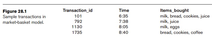
a set of items. A common example is that of market-basket data. Here the market basket corresponds to the sets
of items a consumer buys in a supermarket during one visit. Consider four such
transactions in a random sample shown in Figure 28.1.
An association rule is of the form X => Y, where X = {x1, x2, ..., xn},
and Y = {y1, y2,
..., ym} are sets of items, with xi and yj being distinct items for all i and all j. This
association states that if a customer buys X,
he or she is also likely to buy Y. In
general, any association rule has the form LHS (left-hand side) => RHS
(right-hand side), where LHS and RHS are sets of items. The set LHS ∪ RHS is called an itemset, the set of items purchased by customers. For an
association rule to be of interest to a data miner, the rule should satisfy
some interest measure. Two common interest measures are support and confidence.
The support for a rule LHS => RHS is
with respect to the itemset; it refers to how frequently a specific itemset
occurs in the database. That is, the support is the per-centage of transactions
that contain all of the items in the itemset LHS ∪ RHS. If
the support is low, it implies that there is no overwhelming evidence that
items in LHS ∪ RHS
occur together because the itemset occurs in only a small fraction of
trans-actions. Another term for support is prevalence
of the rule.
The confidence is with regard to the
implication shown in the rule. The confidence of the rule LHS => RHS is
computed as the support(LHS ∪
RHS)/support(LHS). We can think of it as the probability that the items in RHS
will be purchased given that the items in LHS are purchased by a customer.
Another term for confidence is strength of
the rule.
As an
example of support and confidence, consider the following two rules: milk =>
juice and bread => juice. Looking at our four sample transactions in Figure
28.1, we see that the support of {milk, juice} is 50 percent and the support of
{bread, juice} is only 25 percent. The confidence of milk => juice is 66.7
percent (meaning that, of three transactions in which milk occurs, two contain
juice) and the confidence of bread => juice is 50 percent (meaning that one
of two transactions containing bread also contains juice).
As we can
see, support and confidence do not necessarily go hand in hand. The goal of
mining association rules, then, is to generate all possible rules that exceed
some minimum user-specified support and confidence thresholds. The problem is
thus decomposed into two subproblems:
1. Generate
all itemsets that have a support that exceeds the threshold. These sets of
items are called large (or frequent) itemsets. Note that large here means large support.
2. For each large itemset, all the rules that have a
minimum confidence are generated as follows: For a large itemset X and Y ⊂ X, let Z = X – Y; then if sup-port(X)/support(Z) >
minimum confidence, the rule Z => Y (that is, X – Y => Y) is a valid rule.
Generating
rules by using all large itemsets and their supports is relatively
straight-forward. However, discovering all large itemsets together with the
value for their support is a major problem if the cardinality of the set of
items is very high. A typical supermarket has thousands of items. The number of
distinct itemsets is 2m,
where m is the number of items, and
counting support for all possible itemsets becomes very computation intensive.
To reduce the combinatorial search space, algorithms for finding association
rules utilize the following properties:
1. A subset of a large itemset must also be large
(that is, each subset of a large itemset exceeds the minimum required support).
2. Conversely, a superset of a small itemset is
also small (implying that it does not have enough support).
The first
property is referred to as downward
closure. The second property, called the antimonotonicity property, helps to reduce the search space of
possible solutions. That is, once an itemset is found to be small (not a large
itemset), then any extension to that itemset, formed by adding one or more
items to the set, will also yield a small itemset.
2. Apriori Algorithm
The first
algorithm to use the downward closure and antimontonicity properties was the Apriori algorithm, shown as Algorithm
28.1.
We
illustrate Algorithm 28.1 using the transaction data in Figure 28.1 using a
mini-mum support of 0.5. The candidate 1-itemsets are {milk, bread, juice,
cookies, eggs, coffee} and their respective supports are 0.75, 0.5, 0.5, 0.5,
0.25, and 0.25. The first four items qualify for L1 since each support is greater than or equal to 0.5.
In the first iteration of the repeat-loop, we extend the frequent 1-itemsets to
create the candi-date frequent 2-itemsets, C2.
C2 contains {milk, bread},
{milk, juice}, {bread, juice}, {milk, cookies}, {bread, cookies}, and {juice,
cookies}. Notice, for example, that {milk, eggs} does not appear in C2 since {eggs} is small (by
the antimonotonicity property) and does not appear in L1. The supports for the six sets contained in C2 are 0.25, 0.5, 0.25, 0.25,
0.5, and 0.25 and are computed by scanning the set of trans-actions. Only the
second 2-itemset {milk, juice} and the fifth 2-itemset {bread, cookies} have support
greater than or equal to 0.5. These two 2-itemsets form the frequent
2-itemsets, L2.
Algorithm 28.1. Apriori Algorithm for Finding Frequent (Large) Itemsets
Input: Database of m transactions, D, and a minimum support, mins,
represented as a fraction of m.
Output: Frequent itemsets, L1, L2,
..., Lk
Begin /*
steps or statements are numbered for better readability */
Compute support(ij)
= count(ij)/m for each individual item, i1, i2, ..., in
by scanning the database once and counting the number of transactions that item
ij appears in (that is,
count(ij));
The candidate frequent 1-itemset, C1, will be the set of items i1, i2, ..., in;
The subset of items containing ij from C1
where support(ij) >=
mins becomes the frequent
1-itemset,
L1;
k = 1;
termination
= false; repeat
Lk+1 = ;
Create the candidate frequent (k+1)-itemset, Ck+1,
by combining members of Lk
that have k–1 items in common (this
forms candidate frequent (k+1)-itemsets
by selectively extending frequent k-itemsets
by one item);
In addition, only consider as elements of Ck+1 those k+1 items such that every subset of size
k appears in Lk;
Scan the database once and compute the support for
each member of Ck+1;
if the support for a member of Ck+1
>= mins then add that member to Lk+1;
If Lk+1
is empty then termination = true else k =
k + 1;
until termination;
End;
In the
next iteration of the repeat-loop, we construct candidate frequent 3-itemsets
by adding additional items to sets in L2.
However, for no extension of itemsets in L2
will all 2-item subsets be contained in L2.
For example, consider {milk, juice, bread}; the 2-itemset {milk, bread} is not
in L2, hence {milk, juice,
bread} cannot be a frequent 3-itemset by the downward closure property. At
this point the algorithm terminates with L1
equal to {{milk}, {bread}, {juice}, {cookies}} and L2 equal to {{milk, juice}, {bread, cookies}}.
Several
other algorithms have been proposed to mine association rules. They vary mainly
in terms of how the candidate itemsets are generated, and how the supports for
the candidate itemsets are counted. Some algorithms use such data structures as
bitmaps and hashtrees to keep information about itemsets. Several algorithms
have been proposed that use multiple scans of the database because the potential
number of itemsets, 2m,
can be too large to set up counters during a single scan. We will examine three
improved algorithms (compared to the Apriori algorithm) for association rule
mining: the Sampling algorithm, the Frequent-Pattern Tree algorithm, and the
Partition algorithm.
3. Sampling Algorithm
The main idea for the Sampling
algorithm is to select a small sample, one that fits in main memory, of the
database of transactions and to determine the frequent itemsets from that
sample. If those frequent itemsets form a superset of the frequent itemsets for
the entire database, then we can determine the real frequent itemsets by
scanning the remainder of the database in order to compute the exact support
values for the superset itemsets. A superset of the frequent itemsets can
usually be found from the sample by using, for example, the Apriori algorithm,
with a lowered minimum support.
In some rare cases, some frequent itemsets may be missed and a second
scan of the database is needed. To decide whether any frequent itemsets have
been missed, the concept of the negative
border is used. The negative border with respect to a frequent itemset, S, and set of items, I, is the minimal itemsets contained in
PowerSet(I) and not in S. The basic idea is that the negative
border of a set of frequent itemsets contains the closest itemsets that could
also be frequent. Consider the case where a set X is not contained in the frequent itemsets. If all subsets of X are contained in the set of frequent
itemsets, then X would be in the
negative border.
We illustrate this with the following example. Consider the set of items
I = {A, B, C, D, E} and let the
combined frequent itemsets of size 1 to 3 be S = {{A}, {B}, {C}, {D}, {AB}, {AC}, {BC}, {AD}, {CD}, {ABC}}. The
negative border is {{E}, {BD}, {ACD}}. The set {E} is the only 1-itemset not
contained in S, {BD} is the only
2-itemset not in S but whose
1-itemset subsets are, and {ACD} is the only 3-itemset whose 2-itemset subsets
are all in S. The negative border is
important since it is necessary to determine the support for those itemsets in
the negative border to ensure that no large itemsets are missed from analyzing
the sample data.
Support for the negative border is determined when the remainder of the
database is scanned. If we find that an itemset, X, in the negative border belongs in the set of all frequent
itemsets, then there is a potential for a superset of X to also be frequent. If this happens, then a second pass over the
database is needed to make sure that all frequent itemsets are found.
4. Frequent-Pattern
(FP) Tree and FP-Growth Algorithm
The Frequent-Pattern Tree (FP-tree) is
motivated by the fact that Apriori-based algorithms may generate and test a
very large number of candidate itemsets. For example, with 1000 frequent
1-itemsets, the Apriori algorithm would have to generate
or
499,500 candidate 2-itemsets. The FP-Growth
algorithm is one approach that eliminates the generation of a large number
of candidate itemsets.
The
algorithm first produces a compressed version of the database in terms of an
FP-tree (frequent-pattern tree). The FP-tree stores relevant itemset
information and allows for the efficient discovery of frequent itemsets. The
actual mining process adopts a divide-and-conquer strategy where the mining
process is decomposed into a set of smaller tasks that each operates on a
conditional FP-tree, a subset (projection) of the original tree. To start
with, we examine how the FP-tree is constructed. The database is first scanned
and the frequent 1-itemsets along with their support are computed. With this
algorithm, the support is the count
of transactions containing the item rather than the fraction of transactions
containing the item. The frequent 1-itemsets are then sorted in nonincreasing
order of their support. Next, the root of the FP-tree is created with a NULL label. The database is scanned a
second time and for each transaction T
in the database, the frequent 1-itemsets in T
are placed in order as was done with the frequent 1-itemsets. We can designate
this sorted list for T as consisting
of a first item, the head, and the remaining items, the tail. The itemset
information (head, tail) is inserted into the FP-tree recursively, starting at
the root node, as follows:
1. If the current node, N, of the FP-tree has a child with an item name = head, then
increment the count associated with node N
by 1, else create a new node, N, with
a count of 1, link N to its parent
and link N with the item header table
(used for efficient tree traversal).
2. If the tail is nonempty, then repeat step (1) using as the sorted list only the tail, that is, the old head is removed and the new head is the first item from the tail and the remaining items become the new tail.
The item
header table, created during the process of building the FP-tree, contains
three fields per entry for each frequent item: item identifier, support count,
and node link. The item identifier and support count are self-explanatory. The
node link is a pointer to an occurrence of that item in the FP-tree. Since
multiple occurrences of a single item may appear in the FP-tree, these items
are linked together as a list where the start of the list is pointed to by the
node link in the item header table. We illustrate the building of the FP-tree
using the transaction data in Figure 28.1. Let us use a minimum support of 2.
One pass over the four transactions yields the following frequent 1-itemsets
with associated support: {{(milk, 3)}, {(bread, 2)}, {(cookies, 2)}, {(juice,
2)}}. The database is scanned a second time and each transaction will be
processed again.
For the
first transaction, we create the sorted list, T = {milk, bread, cookies, juice}. The items in T are the frequent 1-itemsets from the
first transaction. The items are ordered based on the nonincreasing ordering of
the count of the 1-itemsets found in pass 1 (that is, milk first, bread second,
and so on). We create a NULL root
node for the FP-tree and insert milk
as a child of the root, bread as a
child of milk, cookies as a child of bread,
and juice as a child of cookies. We adjust the entries for the
frequent items in the item header table.
For the
second transaction, we have the sorted list {milk, juice}. Starting at the
root, we see that a child node with label milk
exists, so we move to that node and update
its count
(to account for the second transaction that contains milk). We see that there
is no child of the current node with label juice,
so we create a new node with label juice.
The item header table is adjusted.
The third
transaction only has 1-frequent item, {milk}. Again, starting at the root, we
see that the node with label milk
exists, so we move to that node, increment its count, and adjust the item
header table. The final transaction contains frequent items, {bread, cookies}.
At the root node, we see that a child with label bread does not exist. Thus, we create a new child of the root,
initialize its counter, and then insert cookies
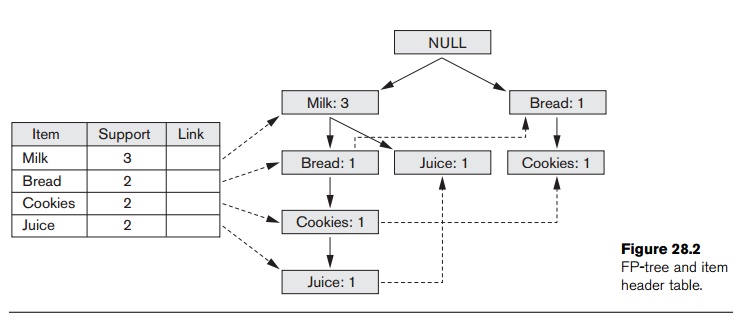
as a child of this node and initialize its count. After the item header table
is updated, we end up with the FP-tree and item header table as shown in Figure
28.2. If we examine this FP-tree, we see that it indeed represents the original
transactions in a compressed format (that is, only showing the items from each
transaction that are large 1-itemsets).
Algorithm
28.2 is used for mining the FP-tree for frequent patterns. With the FP-tree, it
is possible to find all frequent patterns that contain a given frequent item by
starting from the item header table for that item and traversing the node links
in the FP-tree. The algorithm starts with a frequent 1-itemset (suffix pattern)
and con-structs its conditional pattern base and then its conditional FP-tree.
The conditional pattern base is made up of a set of prefix paths, that is,
where the frequent item is a suffix. For example, if we consider the item
juice, we see from Figure 28.2 that there are two paths in the FP-tree that end
with juice: (milk, bread, cookies, juice) and (milk, juice). The two associated
prefix paths are (milk, bread, cookies) and (milk). The conditional FP-tree is
constructed from the patterns in the conditional pattern base. The mining is
recursively performed on this FP-tree. The frequent patterns are formed by
concatenating the suffix pattern with the frequent patterns produced from a
conditional FP-tree.
Algorithm 28.2. FP-Growth Algorithm for Finding
Frequent Itemsets
Input: FP-tree and a minimum support,
mins
Output: frequent patterns (itemsets)
procedure
FP-growth (tree, alpha);
Begin
if tree
contains a single path P then
for each
combination, beta, of the nodes in the path generate pattern (beta ∪ alpha)
with
support = minimum support of nodes in beta
else
for each
item, i, in the header of the tree do
begin
generate
pattern beta = (i ∪ alpha) with support = i.support; construct beta’s conditional pattern base;
construct
beta’s conditional FP-tree, beta_tree; if beta_tree is not empty then
FP-growth(beta_tree,
beta);
end;
End;
We
illustrate the algorithm using the data in Figure 28.1 and the tree in Figure
28.2. The procedure FP-growth is called with the two parameters: the original
FP-tree and NULL for the
variable alpha. Since the original FP-tree has more than a single path, we
execute the else part of the first if statement. We start with the frequent
item, juice. We will examine the frequent items in order of lowest support
(that is, from the last entry in the table to the first). The variable beta is
set to juice with support equal to 2.
Following
the node link in the item header table, we construct the conditional pat-tern
base consisting of two paths (with juice as suffix). These are (milk, bread,
cookies: 1) and (milk: 1). The conditional FP-tree consists of only a single
node, milk: 2. This is due to a support of only 1 for node bread and cookies,
which is below the minimal support of 2. The algorithm is called recursively
with an FP-tree of only a single node (that is, milk: 2) and a beta value of
juice. Since this FP-tree only has one path, all combinations of beta and nodes
in the path are generated—that is, {milk, juice}—with support of 2.
Next, the
frequent item, cookies, is used. The variable beta is set to cookies with
sup-port = 2. Following the node link in the item header table, we construct
the conditional pattern base consisting of two paths. These are (milk, bread:
1) and (bread: 1). The conditional FP-tree is only a single node, bread: 2. The
algorithm is called recursively with an FP-tree of only a single node (that is,
bread: 2) and a beta value of cookies. Since this FP-tree only has one path,
all combinations of beta and nodes in the path are generated, that is, {bread,
cookies} with support of 2. The frequent item, bread, is considered next. The
variable beta is set to bread with support = 2. Following the node link in the
item header table, we construct the conditional pattern base consisting of one
path, which is (milk: 1). The conditional FP-tree is empty since the count is
less than the minimum support. Since the conditional FP-tree is empty, no
frequent patterns will be generated.
The last
frequent item to consider is milk. This is the top item in the item header
table and as such has an empty conditional pattern base and empty conditional
FP-tree. As a result, no frequent patterns are added. The result of executing
the algorithm is the following frequent patterns (or itemsets) with their
support: {{milk: 3}, {bread: 2}, {cookies: 2}, {juice: 2}, {milk, juice: 2},
{bread, cookies: 2}}.
5. Partition Algorithm
Another algorithm, called the Partition
algorithm, is summarized below. If we are given a database with a small
number of potential large itemsets, say, a few thou-sand, then the support for
all of them can be tested in one scan by using a partitioning technique.
Partitioning divides the database into nonoverlapping subsets; these are
individually considered as separate databases and all large itemsets for that
partition, called local frequent
itemsets, are generated in one pass. The Apriori algorithm can then be used
efficiently on each partition if it fits entirely in main memory. Partitions
are chosen in such a way that each partition can be accommodated in main
memory. As such, a partition is read only once in each pass. The only caveat
with the partition method is that the minimum support used for each partition
has a slightly different meaning from the original value. The minimum support
is based on the size of the partition rather than the size of the database for
determining local frequent (large) itemsets. The actual support threshold value
is the same as given earlier, but the support is computed only for a partition.
At the end of pass one, we take the union of all frequent itemsets from
each partition. This forms the global candidate frequent itemsets for the
entire database. When these lists are merged, they may contain some false
positives. That is, some of the itemsets that are frequent (large) in one
partition may not qualify in several other partitions and hence may not exceed
the minimum support when the original database is considered. Note that there
are no false negatives; no large itemsets will be missed. The global candidate
large itemsets identified in pass one are verified in pass two; that is, their
actual support is measured for the entire
database. At the end of phase two, all global large itemsets are identified.
The Partition algorithm lends itself naturally to a parallel or distributed
implementation for better efficiency. Further improvements to this algorithm
have been suggested.
6. Other Types of
Association Rules
Association Rules among Hierarchies. There are
certain types of associations that are
particularly interesting for a special reason. These associations occur among
hierarchies of items. Typically, it is possible to divide items among disjoint
hierarchies based on the nature of the domain. For example, foods in a
supermarket, items in a department store, or articles in a sports shop can be
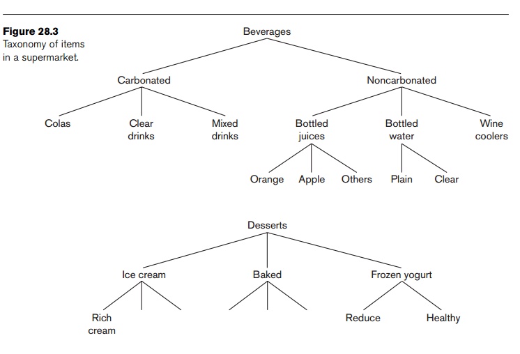
categorized into classes and subclasses that give rise to hierarchies. Consider
Figure 28.3, which shows the taxon-omy of items in a supermarket. The figure
shows two hierarchies—beverages and desserts, respectively. The entire groups
may not produce associations of the form beverages => desserts, or desserts
=> beverages. However, associations of the type Healthy-brand frozen yogurt
=> bottled water, or Rich cream-brand ice cream => wine cooler may
produce enough confidence and support to be valid association rules of
interest.
Therefore,
if the application area has a natural classification of the itemsets into hierarchies,
discovering associations within the
hierarchies is of no particular inter-est. The ones of specific interest are
associations across hierarchies. They
may occur among item groupings at different levels.
Multidimensional Associations. Discovering
association rules involves searching for patterns in a file. In Figure 28.1,
we have an example of a file of customer transactions with three dimensions:
Transaction_id, Time, and Items_bought. However, our data mining tasks and
algorithms introduced up to this point only involve one dimension:
Items_bought. The following rule is an example of including the label of the
single dimension: Items_bought(milk) => Items_bought(juice). It may be of
interest to find association rules that involve multiple dimensions, for
example,
Time(6:30...8:00) => Items_bought(milk). Rules like these are called multidimensional association rules. The
dimensions represent attributes of records
of a file or, in terms of relations, columns of rows of a relation, and can
be categorical or quantitative. Categorical attributes have a finite set of
values that display no ordering relationship. Quantitative attributes are
numeric and their values display an ordering relationship, for example, <.
Items_bought is an example of a categorical attribute and Transaction_id and
Time are quantitative.
One
approach to handling a quantitative attribute is to partition its values into
nonoverlapping intervals that are assigned labels. This can be done in a static
man-ner based on domain-specific knowledge. For example, a concept hierarchy
may group values for Salary into
three distinct classes: low income (0 < Salary <
29,999), middle income (30,000 < Salary <
74,999), and high income (Salary >
75,000). From here, the typical Apriori-type algorithm or one of its variants
can be used for the rule mining since the quantitative attributes now look like
categorical attributes. Another approach to partitioning is to group attribute
values based on data distribution, for example, equidepth partitioning, and
to assign integer values to each partition. The partitioning at this stage may
be relatively fine, that is, a larger number of intervals. Then during the
mining process, these partitions may combine with other adjacent partitions if
their support is less than some predefined maxi-mum value. An Apriori-type
algorithm can be used here as well for the data mining.
Negative Associations. The
problem of discovering a negative association is harder
than that of discovering a positive association. A negative association is of
the following type: 60 percent of
customers who buy potato chips do not buy bottled water. (Here, the 60 percent refers to the confidence for the
negative association rule.) In a
database with 10,000 items, there are 210,000 possible combinations of items, a
majority of which do not appear even once in the database. If the absence of a
certain item combination is taken to mean a negative association, then we
potentially have millions and millions of negative association rules with RHSs
that are of no interest at all. The problem, then, is to find only interesting negative rules. In general,
we are interested in cases in which two specific sets of items appear very
rarely in the same transaction. This poses two problems.
1. For a total item inventory of 10,000 items, the
probability of any two being bought together is (1/10,000) *
(1/10,000) = 10–8. If we find the actual sup-port for these two
occurring together to be zero, that does not represent a significant departure
from expectation and hence is not an interesting (negative) association.
2. The other
problem is more serious. We are looking for item combinations with very low
support, and there are millions and millions with low or even zero support. For
example, a data set of 10 million transactions has most of the 2.5 billion
pairwise combinations of 10,000 items missing. This would generate billions of
useless rules.
Therefore,
to make negative association rules interesting, we must use prior knowledge
about the itemsets. One approach is to use hierarchies. Suppose we use the
hierarchies of soft drinks and chips shown in Figure 28.4.
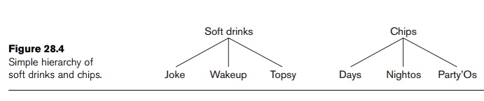
A strong positive association has been shown between soft drinks and chips. If we find a large support for the fact that when customers buy Days chips they predominantly buy Topsy and not Joke and not Wakeup, that would be interesting because we would normally expect that if there is a strong association between Days and Topsy, there should also be such a strong association between Days and Joke or Days and Wakeup.
In the
frozen yogurt and bottled water groupings shown in Figure 28.3, suppose the
Reduce versus Healthy-brand division is 80–20 and the Plain and Clear brands
division is 60–40 among respective categories. This would give a joint
probability of Reduce frozen yogurt being purchased with Plain bottled water as
48 percent among the transactions containing a frozen yogurt and bottled water.
If this sup-port, however, is found to be only 20 percent, it would indicate a
significant negative association among Reduce yogurt and Plain bottled water;
again, that would be interesting.
The
problem of finding negative association is important in the above situations
given the domain knowledge in the form of item generalization hierarchies (that
is, the beverage given and desserts hierarchies shown in Figure 28.3), the
existing positive associations (such as between the frozen yogurt and bottled
water groups), and the distribution of items (such as the name brands within
related groups). The scope of discovery of negative associations is limited in
terms of knowing the item hierarchies and distributions. Exponential growth of
negative associations remains a challenge.
7. Additional
Considerations for Association Rules
Mining association rules in real-life databases is complicated by the
following fac-tors:
The cardinality of itemsets in
most situations is extremely large, and the volume of transactions is very
high as well. Some operational databases in retailing and communication
industries collect tens of millions of transactions per day.
1. Transactions show variability in such factors as geographic location and sea-sons, making sampling difficult.
2. Item classifications exist
along multiple dimensions. Hence, driving the discovery process with domain
knowledge, particularly for negative rules, is extremely difficult.
3.Quality of data is variable;
significant problems exist with missing, erroneous, conflicting, as well as
redundant data in many industries.
Related Topics