Sample rates and size: Irregular sampling errors, Nyquist’s theorem

Sample rates and size

So far, much of the discussion has been on the sample size. Another important parameter is the sampling rate. The sampling rate is the number of samples that are taken in a time period, usually one second, and is normally measured in hertz, in the same way that frequencies are measured. This determines several aspects of the conversion process:

It determines the speed of the conversion device itself. All converters require a certain amount of time to perform the conversion and this conversion time determines the maxi-mum rate at which samples can be taken. Needless to say, the fast converters tend to be the more expensive ones.

•                                                                         The sample rate determines the maximum frequency that can be converted. This is explained later in the section on Nyquist’s theorem.

•                                                                         Sampling must be performed on a regular basis with ex-actly the same time period between samples. This is impor-tant to remove conversion errors due to irregular sampling.

Irregular sampling errors

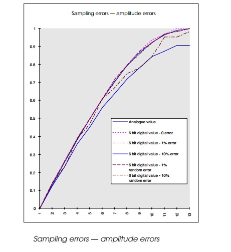
The line chart shows the effect of irregular sampling. It effectively alters the amplitude or magnitude of the analogue signal being measured. With reference to the curve in the chart, the following errors can occur:

•                                                                         If the sample is taken early, the value converted will be less than it should be. Quantisation errors will then be added to compound the error.

•                                                                         If the sample is taken late, the value will be higher than expected. If all or the majority of the samples are taken early, the curve is reproduced with a similar general shape but with a lower amplitude. One important fact is that the sampled curve will not reflect the peak amplitudes that the original curve will have.

•                                                                         If there is a random timing error — often called jitter — then the resulting curve is badly distorted, again as shown in the chart.

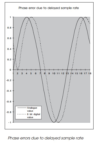
Other sample rate errors can be introduced if there is a delay in getting the samples. If the delay is constant, the correct charac-teristics for the curve are obtained but out of phase. It is interesting that there will always be a phase error due to the conversion time taken by the converter. The conversion time will delay the digital output and therefore introduces the phase error — but this is usually very small and can typically be ignored.

The phase error shown assumes that all delays are consist-ent. If this is not the case, different curves can be obtained as shown in the next chart. Here the samples have been taken at random and at slightly delayed intervals. Both return a similar curve to that of the original value — but still with significant errors.

In summary, it is important that samples are taken on a regular basis with consistent intervals between them. Failure to observe these design conditions will introduce errors. For this reason, many microprocessor-based implementations use a timer and interrupt service routine mechanism to gather samples. The timer is set-up to generate an interrupt to the processor at the sampling rate frequency. Every time the interrupt occurs, the interrupt service routine reads the last value for the converter and instructs it to start a new conversion before returning to normal execution. The instructions always take the same amount of time and therefore sampling integrity is maintained.

Nyquist’s theorem

The sample rate also must be chosen carefully when consid-ering the maximum frequency of the analogue signal being con-verted. Nyquist’s theorem states that the minimum sampling rate frequency should be twice the maximum frequency of the ana-logue signal. A 4 kHz analogue signal would need to be sampled at twice that frequency to convert it digitally. For example, a hi-fi audio signal with a frequency range of 20 to 20 kHz would need a minimum sampling rate of 40 kHz.

Higher frequency sampling introduces a frequency compo-nent which is normally filtered out using an analogue filter.