Classification - Data Mining

Classification

Classification is the process of learning a model that describes different classes of data. The classes are predetermined. For example, in a banking application, customers who apply for a credit card may be classified as a poor risk, fair risk, or good risk. Hence this type of activity is also called supervised learning. Once the model is built, it can be used to classify new data. The first step—learning the model—is accomplished by using a training set of data that has already been classified. Each record in the training data contains an attribute, called the class label, which indicates which class the record belongs to. The model that is produced is usually in the form of a decision tree or a set of rules. Some of the important issues with regard to the model and the algorithm that produces the model include the model’s ability to predict the correct class of new data, the computational cost associated with the algorithm, and the scalability of the algorithm.

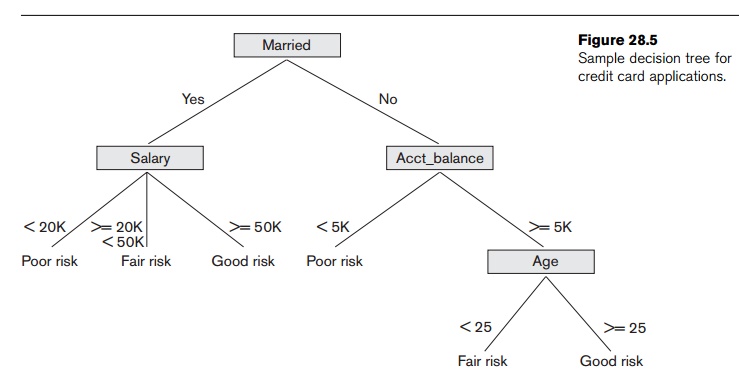
We will examine the approach where our model is in the form of a decision tree. A decision tree is simply a graphical representation of the description of each class or, in other words, a representation of the classification rules. A sample decision tree is pictured in Figure 28.5. We see from Figure 28.5 that if a customer is married and if salary >= 50K, then they are a good risk for a bank credit card. This is one of the rules that describe the class good risk. Traversing the decision tree from the root to each leaf node forms other rules for this class and the two other classes. Algorithm 28.3 shows the procedure for constructing a decision tree from a training data set. Initially, all training samples are at the root of the tree. The samples are partitioned

recursively based on selected attributes. The attribute used at a node to partition the samples is the one with the best splitting criterion, for example, the one that maximizes the information gain measure.

Algorithm 28.3. Algorithm for Decision Tree Induction

Input: Set of training data records: R₁, R₂, ..., R_m and set of attributes: A₁, A₂, ..., A_n

Output: Decision tree

procedure Build_tree (records, attributes);

Begin

create a node N;

if all records belong to the same class, C then return N as a leaf node with class label C;

if attributes is empty then

return N as a leaf node with class label C, such that the majority of records belong to it;

select attribute A_i (with the highest information gain) from attributes; label node N with A_i;

for each known value, v_j, of A_i do

begin

add a branch from node N for the condition A_i = v_j; S_j = subset of records where A_i = v_j;

if S_j is empty then

add a leaf, L, with class label C, such that the majority of records belong to it and return L

else add the node returned by Build_tree(S_j, attributes – A_i);

end;

End;

Before we illustrate Algorithm 28.3, we will explain the information gain measure in more detail. The use of entropy as the information gain measure is motivated by the goal of minimizing the information needed to classify the sample data in the resulting partitions and thus minimizing the expected number of conditional tests needed to classify a new record. The expected information needed to classify training data of s samples, where the Class attribute has n values (v₁, ..., v_n) and s_i is the number of samples belonging to class label v_i, is given by

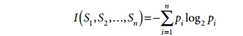
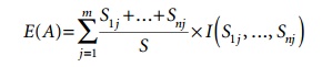
where p_i is the probability that a random sample belongs to the class with label v_i. An estimate for p_i is s_i /s. Consider an attribute A with values {v₁, ..., v_m} used as the test attribute for splitting in the decision tree. Attribute A partitions the samples into the subsets S₁, ..., S_m where samples in each S_j have a value of v_j for attribute A. Each S_j may contain samples that belong to any of the classes. The number of samples in S_j that belong to class i can be denoted as s_ij. The entropy associated with using attribute A as the test attribute is defined as

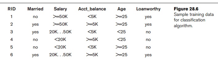
I(s_1j, ..., s_nj) can be defined using the formulation for I(s₁, ..., s_n) with p _i being replaced by p_ij where p_ij = s_ij /s_j. Now the information gain by partitioning on attrib-ute A, Gain(A), is defined as I(s₁, ..., s_n) – E(A). We can use the sample training data from Figure 28.6 to illustrate the algorithm.

The attribute RID represents the record identifier used for identifying an individual record and is an internal attribute. We use it to identify a particular record in our example. First, we compute the expected information needed to classify the training data of 6 records as I(s₁, s₂) where there are two classes: the first class label value cor-responds to yes and the second to no. So,

I(3,3) = − 0.5log₂ 0.5 − 0.5log₂ 0.5 = 1.

Now, we compute the entropy for each of the four attributes as shown below. For

Married = yes, we have s₁₁ = 2, s₂₁ = 1 and I(s₁₁, s₂₁) = 0.92. For Married = no, we have s₁₂ = 1, s₂₂ = 2 and I(s₁₂, s₂₂) = 0.92. So, the expected information needed to classify

a sample using attribute Married as the partitioning attribute is

E(Married) = 3/6 I(s₁₁, s₂₁) + 3/6 I(s₁₂, s₂₂) = 0.92.

The gain in information, Gain(Married), would be 1 – 0.92 = 0.08. If we follow simi-lar steps for computing the gain with respect to the other three attributes we end up with

E(Salary) = 0.33   and    Gain(Salary) = 0.67

E(Acct_balance) = 0.92 and    Gain(Acct_balance) = 0.08

E(Age) = 0.54       and    Gain(Age) = 0.46

Since the greatest gain occurs for attribute Salary, it is chosen as the partitioning attribute. The root of the tree is created with label Salary and has three branches, one for each value of Salary. For two of the three values, that is, <20K and >=50K, all the samples that are partitioned accordingly (records with RIDs 4 and 5 for <20K

and records with RIDs 1 and 2 for >=50K) fall within the same class loanworthy no and loanworthy yes respectively for those two values. So we create a leaf node for each. The only branch that needs to be expanded is for the value 20K...50K with two samples, records with RIDs 3 and 6 in the training data. Continuing the process using these two records, we find that Gain(Married) is 0, Gain(Acct_balance) is 1, and Gain(Age) is 1.

We can choose either Age or Acct_balance since they both have the largest gain. Let us choose Age as the partitioning attribute. We add a node with label Age that has two branches, less than 25, and greater or equal to 25. Each branch partitions the remaining sample data such that one sample record belongs to each branch and hence one class. Two leaf nodes are created and we are finished. The final decision tree is pictured in Figure 28.7.