Data Modeling for Data Warehouses

Data Modeling for Data Warehouses

Multidimensional models take advantage of inherent relationships in data to populate data in multidimensional matrices called data cubes. (These may be called hypercubes if they have more than three dimensions.) For data that lends itself to dimensional formatting, query performance in multidimensional matrices can be much better than in the relational data model. Three examples of dimensions in a corporate data warehouse are the corporation’s fiscal periods, products, and regions.

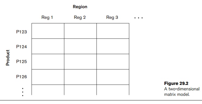
A standard spreadsheet is a two-dimensional matrix. One example would be a spreadsheet of regional sales by product for a particular time period. Products could be shown as rows, with sales revenues for each region comprising the columns. (Figure 29.2 shows this two-dimensional organization.) Adding a time dimension,

such as an organization’s fiscal quarters, would produce a three-dimensional matrix, which could be represented using a data cube.

Figure 29.3 shows a three-dimensional data cube that organizes product sales data by fiscal quarters and sales regions. Each cell could contain data for a specific product,

specific fiscal quarter, and specific region. By including additional dimensions, a data hypercube could be produced, although more than three dimensions cannot be easily visualized or graphically presented. The data can be queried directly in any combination of dimensions, bypassing complex database queries. Tools exist for viewing data according to the user’s choice of dimensions.

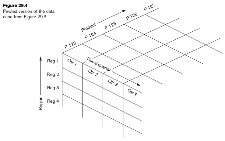
Changing from one-dimensional hierarchy (orientation) to another is easily accomplished in a data cube with a technique called pivoting (also called rotation). In this technique the data cube can be thought of as rotating to show a different orientation of the axes. For example, you might pivot the data cube to show regional sales revenues as rows, the fiscal quarter revenue totals as columns, and the company’s products in the third dimension (Figure 29.4). Hence, this technique is equivalent to having a regional sales table for each product separately, where each table shows quarterly sales for that product region by region.

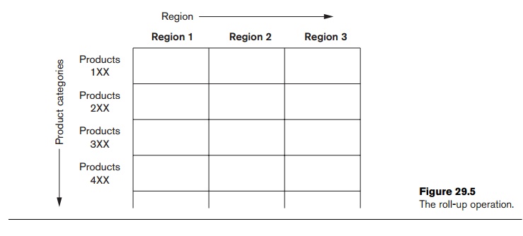
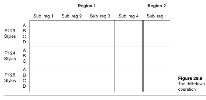
Multidimensional models lend themselves readily to hierarchical views in what is known as roll-up display and drill-down display. A roll-up display moves up the hierarchy, grouping into larger units along a dimension (for example, summing weekly data by quarter or by year). Figure 29.5 shows a roll-up display that moves from individual products to a coarser-grain of product categories. Shown in Figure 29.6, a drill-down display provides the opposite capability, furnishing a finer-grained view, perhaps disaggregating country sales by region and then regional sales by subregion and also breaking up products by styles.

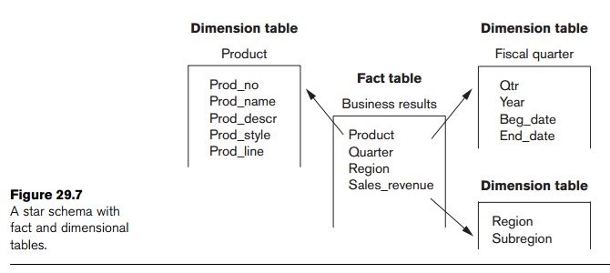
The multidimensional storage model involves two types of tables: dimension tables and fact tables. A dimension table consists of tuples of attributes of the dimension. A fact table can be thought of as having tuples, one per a recorded fact. This fact contains some measured or observed variable(s) and identifies it (them) with pointers to dimension tables. The fact table contains the data, and the dimensions identify each tuple in that data. Figure 29.7 contains an example of a fact table that can be viewed from the perspective of multiple dimension tables.

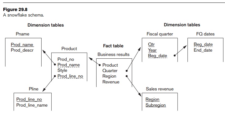
Two common multidimensional schemas are the star schema and the snowflake schema. The star schema consists of a fact table with a single table for each dimension (Figure 29.7). The snowflake schema is a variation on the star schema in which

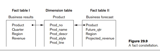
the dimensional tables from a star schema are organized into a hierarchy by normalizing them (Figure 29.8). Some installations are normalizing data warehouses up to the third normal form so that they can access the data warehouse to the finest level of detail. A fact constellation is a set of fact tables that share some dimension tables. Figure 29.9 shows a fact constellation with two fact tables, business results and business forecast. These share the dimension table called product. Fact constellations limit the possible queries for the warehouse.

Data warehouse storage also utilizes indexing techniques to support high-performance access (see Chapter 18 for a discussion of indexing). A technique called bitmap indexing constructs a bit vector for each value in a domain (column)

being indexed. It works very well for domains of low cardinality. There is a 1 bit placed in the jth position in the vector if the jth row contains the value being indexed. For example, imagine an inventory of 100,000 cars with a bitmap index on car size. If there are four car sizes—economy, compact, mid-size, and full-size— there will be four bit vectors, each containing 100,000 bits (12.5K) for a total index size of 50K. Bitmap indexing can provide considerable input/output and storage space advantages in low-cardinality domains. With bit vectors a bitmap index can provide dramatic improvements in comparison, aggregation, and join performance.

In a star schema, dimensional data can be indexed to tuples in the fact table by join indexing. Join indexes are traditional indexes to maintain relationships between primary key and foreign key values. They relate the values of a dimension of a star schema to rows in the fact table. For example, consider a sales fact table that has city and fiscal quarter as dimensions. If there is a join index on city, for each city the join index maintains the tuple IDs of tuples containing that city. Join indexes may involve multiple dimensions.

Data warehouse storage can facilitate access to summary data by taking further advantage of the nonvolatility of data warehouses and a degree of predictability of the analyses that will be performed using them. Two approaches have been used: (1) smaller tables including summary data such as quarterly sales or revenue by product line, and (2) encoding of level (for example, weekly, quarterly, annual) into existing tables. By comparison, the overhead of creating and maintaining such aggregations would likely be excessive in a volatile, transaction-oriented database.