Collective Communication

COLLECTIVE COMMUNICATION

 

If we pause for a moment and think about our trapezoidal rule program, we can find several things that we might be able to improve on. One of the most obvious is that the “global sum” after each process has computed its part of the integral. If we hire eight workers to, say, build a house, we might feel that we weren’t getting our money’s worth if seven of the workers told the first what to do, and then the seven collected their pay and went home. But this is very similar to what we’re doing in our global sum. Each process with rank greater than 0 is “telling process 0 what to do” and then quitting. That is, each process with rank greater than 0 is, in effect, saying “add this number into the total.” Process 0 is doing nearly all the work in computing the global sum, while the other processes are doing almost nothing. Sometimes it does happen that this is the best we can do in a parallel program, but if we imagine that we have eight students, each of whom has a number, and we want to find the sum of all eight numbers, we can certainly come up with a more equitable distribution of the work than having seven of the eight give their numbers to one of the students and having the first do the addition.

 

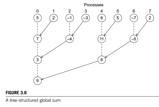
1. Tree-structured communication

 

As we already saw in Chapter 1 we might use a “binary tree structure” like that illustrated in Figure 3.6. In this diagram, initially students or processes 1, 3, 5, and 7 send their values to processes 0, 2, 4, and 6, respectively. Then processes 0, 2, 4, and 6 add the received values to their original values, and the process is repeated twice:

 

        a.  Processes 2 and 6 send their new values to processes 0 and 4, respectively.

 

        b. Processes 0 and 4 add the received values into their new values.

 

        a.  Process 4 sends its newest value to process 0.

 

        b. Process 0 adds the received value to its newest value.

 

This solution may not seem ideal, since half the processes (1, 3, 5, and 7) are doing the same amount of work that they did in the original scheme. However, if you think about it, the original scheme required comm_sz-1 = seven receives and seven adds by process 0, while the new scheme only requires three, and all the other processes do no more than two receives and adds. Furthermore, the new scheme has a property by which a lot of the work is done concurrently by different processes. For example, in the first phase, the receives and adds by processes 0, 2, 4, and 6 can all take place simultaneously. So, if the processes start at roughly the same time, the total time required to compute the global sum will be the time required by process 0, that is, three receives and three additions. We’ve thus reduced the overall time by more than 50%. Furthermore, if we use more processes, we can do even better. For example, if comm_sz = 1024, then the original scheme requires process 0 to do 1023 receives and additions, while it can be shown (Exercise 3.5) that the new scheme requires process 0 to do only 10 receives and additions. This improves the original scheme by more than a factor of 100!

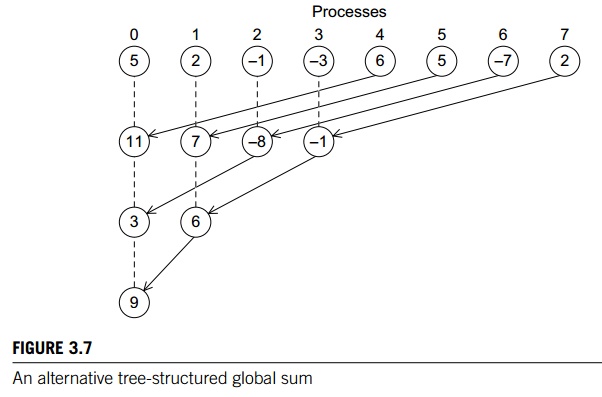
You may be thinking to yourself, this is all well and good, but coding this tree-structured global sum looks like it would take a quite a bit of work, and you’d be right. See Programming Assignment 3.3. In fact, the problem may be even harder. For example, it’s perfectly feasible to construct a tree-structured global sum that uses different “process-pairings.” For example, we might pair 0 and 4, 1 and 5, 2 and 6, and 3 and 7 in the first phase. Then we could pair 0 and 2, and 1 and 3 in the second, and 0 and 1 in the final. See Figure 3.7. Of course, there are many other possibilities. How can we decide which is the best? Do we need to code each alternative and evaluate its performance? If we do, is it possible that one method works best for “small” trees, while another works best for “large” trees? Even worse, one approach might work best on system A, while another might work best on system B.

 

2. MPI_Reduce

With virtually limitless possibilities, it’s unreasonable to expect each MPI pro-grammer to write an optimal global-sum function, so MPI specifically protects programmers against this trap of endless optimization by requiring that MPI imple-mentations include implementations of global sums. This places the burden of optimization on the developer of the MPI implementation, rather than the applica-tion developer. The assumption here is that the developer of the MPI implementation should know enough about both the hardware and the system software so that she can make better decisions about implementation details.

 

Now, a “global-sum function” will obviously require communication. However, unlike the MPI_Send-MPI Recv pair, the global-sum function may involve more than two processes. In fact, in our trapezoidal rule program it will involve all the processes in MPI_COMM WORLD. In MPI parlance, communication functions that involve all the processes in a communicator are called collective communications. To distinguish between collective communications and functions such as MPI_Send and MPI_Recv, MPI_Send and MPI_Recv are often called point-to-point communications.

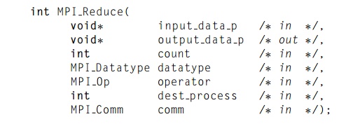
In fact, global sum is just a special case of an entire class of collective communi-cations. For example, it might happen that instead of finding the sum of a collection of comm_sz numbers distributed among the processes, we want to find the maximum or the minimum or the product or any one of many other possibilities. MPI generalized the global-sum function so that any one of these possibilities can be implemented with a single function:

The key to the generalization is the fifth argument, operator. It has type MPI_Op, which is a predefined MPI type like MPI_Datatype and MPI_Comm. There are a number of predefined values in this type. See Table 3.2. It’s also possible to define your own operators; for details, see the MPI-1 Standard [39].

The operator we want is MPI_SUM. Using this value for the operator argument, we can replace the code in Lines 18 through 28 of Program 3.2 with the single function call MPI_Reduce(&local_int, &total_int, 1, MPI_DOUBLE, MPI_SUM, 0, MPI_COMM_WORLD);

 

One point worth noting is that by using a count argument greater than 1, MPI_Reduce can operate on arrays instead of scalars. The following code could thus be used to

add a collection of N-dimensional vectors, one per process:

double local_x[N], sum[N];

 

. . .

 

MPI_Reduce(local_x, sum, N, MPI_DOUBLE, MPI_SUM, 0, MPI_COMM_WORLD);

 3. Collective vs. point-to-point communications

 

It’s important to remember that collective communications differ in several ways from point-to-point communications:

 

      1. All the processes in the communicator must call the same collective function. For example, a program that attempts to match a call to MPI_Reduce on one process with a call to MPI_Recv on another process is erroneous, and, in all likelihood, the program will hang or crash.

         2. The arguments passed by each process to an MPI collective communication must be “compatible.” For example, if one process passes in 0 as the dest_process and another passes in 1, then the outcome of a call to MPI_Reduce is erroneous, and, once again, the program is likely to hang or crash.

         3. The output data p argument is only used on dest_process. However, all of the processes still need to pass in an actual argument corresponding to output_data_p, even if it’s just NULL.

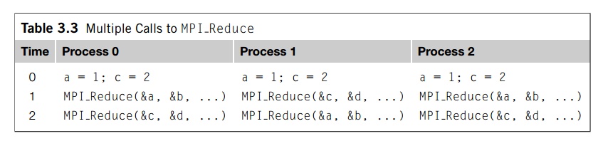
      4. Point-to-point communications are matched on the basis of tags and communica-tors. Collective communications don’t use tags, so they’re matched solely on the basis of the communicator and the order in which they’re called. As an example, consider the calls to MPI Reduce shown in Table 3.3. Suppose that each pro-cess calls MPI Reduce with operator MPI_SUM, and destination process 0. At first glance, it might seem that after the two calls to MPI_Reduce, the value of b will be three, and the value of d will be six. However, the names of the memory locations are irrelevant to the matching, of the calls to MPI_Reduce. The order of the calls will determine the matching, so the value stored in b will be 1 + 2 + 1 = 4, and the value stored in d will be 2 + 1 + 2 = 5.

       

          4. P

A final caveat: it might be tempting to call MPI_Reduce using the same buffer for both input and output. For example, if we wanted to form the global sum of x on each process and store the result in x on process 0, we might try calling

MPI_Reduce(&x, &x, 1, MPI_DOUBLE, MPI_SUM, 0, comm);

Table 3.3 Multiple Calls to MPI_Reduce

However, this call is illegal in MPI, so its result will be unpredictable: it might pro-

 

duce an incorrect result, it might cause the program to crash, it might even produce a correct result. It’s illegal because it involves aliasing of an output argument. Two arguments are aliased if they refer to the same block of memory, and MPI prohibits aliasing of arguments if one of them is an output or input/output argument. This is because the MPI Forum wanted to make the Fortran and C versions of MPI as sim-ilar as possible, and Fortran prohibits aliasing. In some instances, MPI provides an alternative construction that effectively avoids this restriction. See Section 6.1.9 for an example.

 

4. MPI_Allreduce

In our trapezoidal rule program, we just print the result, so it’s perfectly natural for only one process to get the result of the global sum. However, it’s not difficult to imagine a situation in which all of the processes need the result of a global sum in order to complete some larger computation. 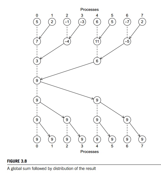In this situation, we encounter some of the same problems we encountered with our original global sum. For example, if we use a tree to compute a global sum, we might “reverse” the branches to distribute the global sum (see Figure 3.8). Alternatively, we might have the processes exchange partial results instead of using one-way communications. Such a communication pat-tern is sometimes called a butterfly (see Figure 3.9). Once again, we don’t want to have to decide on which structure to use, or how to code it for optimal performance. Fortunately, MPI provides a variant of MPI Reduce that will store the result on all the processes in the communicator:

int MPI_Allreduce(

void* input_data_p

void* output_data_p

int        count

MPI_Datatype datatype

MPI_Op           operator

MPI_Comm     comm.

The argument list is identical to that for MPI_Reduce except that there is no dest_process since all the processes should get the result.

 

5. Broadcast

 

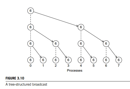
If we can improve the performance of the global sum in our trapezoidal rule program by replacing a loop of receives on process 0 with a tree-structured communication, we ought to be able to do something similar with the distribution of the input data. In fact, if we simply “reverse” the communications in the tree-structured global sum in Figure 3.6, we obtain the tree-structured communication shown in Figure 3.10, and we can use this structure to distribute the input data. A collective communication in which data belonging to a single process is sent to all of the processes in the communicator is called a broadcast, and you’ve probably guessed that MPI provides

 a broadcast function:

int MPI Bcast(

void* data p         /* in/out     */,

int     count /*       in       */,

MPI_Datatype datatype          /*       in       */,

int     source proc /*       in       */,

MPI_Comm         comm          /*       in       */);

The process with rank source proc sends the contents of the memory referenced by data p to all the processes in the communicator comm. Program 3.6 shows how to modify the Get input function shown in Program 3.5 so that it uses MPI Bcast instead of MPI Send and MPI Recv.

Program 3.6: A version of Get input that uses MPI Bcast

          void Get input(

          int     my_rank     /*       in       */,

          int     comm_sz    /*       in       */,

          double         a_p    / * out  */,

          double         b_p   /*  out  */,

          int     n_p   /*       out  */) {

          if (my_rank == 0) {

          printf("Enter a, b, and nnn");

          scanf("%lf %lf %d", a p, b p, n p);

          }

          MPI Bcast(a_p, 1, MPI_DOUBLE, 0, MPI_COMM_WORLD);

          MPI Bcast(b_p, 1, MPI_DOUBLE, 0, MPI_COMM_WORLD);

          MPI Bcast(n_p, 1, MPI_INT, 0, MPI_COMM_WORLD);

          }  /*  Get input  */

Recall that in serial programs, an in/out argument is one whose value is both used and changed by the function. For MPI Bcast, however, the data p argument is an input argument on the process with rank source proc and an output argument on the other processes. Thus, when an argument to a collective communication is labeled in/out, it’s possible that it’s an input argument on some processes and an output argument on other processes.

6. Data distributions

 

Suppose we want to write a function that computes a vector sum:

 

x + y = (x₀, x₁,….., x_n-₁) +(.y₀, y₁, …., y_n-₁)

 

        =(x₀ + y₀, x₁ + y₁,….., x_n-₁ + y_n -₁)

        =(z₀, z₁,….., z_n-₁)

 

        = z

 

If we implement the vectors as arrays of, say, doubles, we could implement serial vector addition with the code shown in Program 3.7.

Program 3.7: A serial implementation of vector addition

            void Vector_sum(double x[], double y[], double z[], int n) {

            int        i;

            for       (i = 0; i < n; i++)

                        z[i] = x[i] + y[i];

            }  /*  Vector sum  */

          How could we implement this using MPI? The work consists of adding the indi-vidual components of the vectors, so we might specify that the tasks are just the additions of corresponding components. Then there is no communication between the tasks, and the problem of parallelizing vector addition boils down to aggregat-ing the tasks and assigning them to the cores. If the number of components is n and we have comm sz cores or processes, let’s assume that n evenly divides comm sz and define local_n = n/comm._sz. Then we can simply assign blocks of local n consec-utive components to each process. The four columns on the left of Table 3.4 show an example when n = 12 and comm._sz = 3. This is often called a block partition of the vector.

An alternative to a block partition is a cyclic partition. In a cyclic partition, we assign the components in a round robin fashion. The four columns in the mid-dle of Table 3.4 show an example when n = 12 and comm._sz = 3. Process 0 gets component 0, process 1 gets component 1, process 2 gets component 2, process 0 gets component 3, and so on.

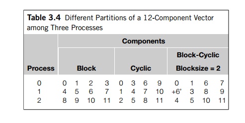
A third alternative is a block-cyclic partition. The idea here is that instead of using a cyclic distribution of individual components, we use a cyclic distri-bution of blocks of components, so a block-cyclic distribution isn’t fully spec-ified until we decide how large the blocks are. If comm _sz = 3, n = 12, and the blocksize b = 2, an example is shown in the four columns on the right of Table 3.4.

Once we’ve decided how to partition the vectors, it’s easy to write a parallel vector addition function: each process simply adds its assigned components. Furthermore, regardless of the partition, each process will have local_n components of the vec-tor, and, in order to save on storage, we can just store these on each process as an array of local_n elements. Thus, each process will execute the function shown in Program 3.8. Although the names of the variables have been changed to emphasize the fact that the function is operating on only the process’ portion of the vector, this function is virtually identical to the original serial function.

Program 3.8: A parallel implementation of vector addition

          void Parallel_vector_sum(

          double         local_x[]     /*       in       */,

          double         local_y[]     /*       in       */,

          double         local_z[]      /*       out    */,

          int     local_n        /*       in       */) {

          int local_i;                     

          for (local_i = 0; local_i < local_n; local i++)

          local_z[local i] = local_x[local i] + local_y[local i];

          }  /*  Parallel vector sum  */

7. Scatter

Now suppose we want to test our vector addition function. It would be convenient to be able to read the dimension of the vectors and then read in the vectors x and y.

We already know how to read in the dimension of the vectors: process 0 can prompt the user, read in the value, and broadcast the value to the other processes. We might try something similar with the vectors: process 0 could read them in and broadcast them to the other processes. However, this could be very wasteful. If there are 10 processes and the vectors have 10,000 components, then each process will need to allocate storage for vectors with 10,000 components, when it is only operating on subvectors with 1000 components. If, for example, we use a block distribution, it would be better if process 0 sent only components 1000 to 1999 to process 1, components 2000 to 2999 to process 2, and so on. Using this approach, processes 1 to 9 would only need to allocate storage for the components they’re actually using.

 

Thus, we might try writing a function that reads in an entire vector that is on process 0 but only sends the needed components to each of the other processes. For the communication MPI provides just such a function:

int MPI Scatter(

void   send_buf_p /*       in       */,

int     send_count /*       in       */,

MPI_Datatype     send_type   /*       in       */,

void   recv_buf_p /*       out    */,

int     recv_count  /*       in       */,

MPI_Datatype     recv_type    /*       in       */,

int     src_proc     /*       in       */,

MPI_Comm         comm          /*       in       */);

If the communicator comm contains comm_sz processes, then MPI_Scatter divides the data referenced by send buf p into comm_sz pieces—the first piece goes to process 0, the second to process 1, the third to process 2, and so on. For example, suppose we’re using a block distribution and process 0 has read in all of an n-component vector into send_buf p. Then, process 0 will get the first local_n = n=comm_sz components, process 1 will get the next local n components, and so on. Each process should pass its local vector as the recv buf p argument and the recv_count argument should be local_n. Both send_type and recv_type should be MPI_DOUBLE and src_proc should be 0. Perhaps surprisingly, send_count should also be local n—send count is the amount of data going to each process; it’s not the amount of data in the memory referred to by send_buf_p. If we use a block distribution and MPI_Scatter, we can read in a vector using the function Read_vector shown in Program 3.9.

 

One point to note here is that MPI_Scatter sends the first block of send count objects to process 0, the next block of send_count objects to process 1, and so on, so this approach to reading and distributing the input vectors will only be suitable if we’re using a block distribution and n, the number of components in the vectors, is evenly divisible by comm_sz. We’ll discuss a partial solution to dealing with a cyclic or block-cyclic distribution in Exercise 18. For a complete solution, see. We’ll look at dealing with the case in which n is not evenly divisible by comm sz in Exercise 3.13.

Program 3.9: A function for reading and distributing a vector

 

          void Read vector(

          double         local_a[]      /*       out    */,

          int     local_n        /*       in       */,

          int     n        /*       in       */,

          char   vec_name[] /*       in       */,

          int     my_rank     /*       in       */,

          MPI_Comm         comm          /*       in       */) {

          double  a = NULL;

          int i;

          if (my_rank == 0) {

          a = malloc(n sizeof(double));

          printf("Enter the vector %snn", vec name);

          for (i = 0; i < n; i++)

          scanf("%lf", &a[i]);

          MPI_Scatter(a, local n, MPI DOUBLE, local a, local n,

          MPI_DOUBLE, 0, comm);

          free(a);

          } else {

          MPI Scatter(a, local_n, MPI_DOUBLE, local_a, local_n,

          MPI_DOUBLE, 0, comm);

          }

          }  /*  Read vector  */

 

8. Gather

Of course, our test program will be useless unless we can see the result of our vector addition, so we need to write a function for printing out a distributed vector. Our function can collect all of the components of the vector onto process 0, and then process 0 can print all of the components. The communication in this function can be carried out by MPI_Gather,

int MPI_Gather(

void   send_buf_p /*       in       */,

int     send_count /*       in       */,

MPI_Datatype     send_type   /*       in       */,

void   recv_buf_p /*       out    */,

int     recv_count  /*       in       */,

MPI_Datatype     recv_type    /*       in       */,

int     dest_proc    /*       in       */,

MPI_Comm         comm          /*       in       */);

The data stored in the memory referred to by send buf p on process 0 is stored in the first block in recv buf p, the data stored in the memory referred to by send buf p on process 1 is stored in the second block referred to by recv buf p, and so on. So, if we’re using a block distribution, we can implement our distributed vector print function as shown in Program 3.10. Note that recv count is the number of data items received from each process, not the total number of data items received.

Program 3.10: A function for printing a distributed vector

          void Print_vector(

          double         local_b[]     /*  in  */,

          int     local_n        /*  in  */,

          int     n        /*  in  */,

          char   title[] /*  in  */,

          int     my_rank     /*  in  */,

          MPI_Comm         comm          /*  in  */) {

          double  b = NULL;

          int i;

          if (my_rank == 0) {

          b = malloc(n sizeof(double));

          MPI_Gather(local_b, local_n, MPI_DOUBLE, b, local n,

          MPI_DOUBLE, 0, comm);

          printf("%snn", title);

          for (i = 0; i < n; i++)

          printf("%f ", b[i]);

          printf("\n");

          free(b);

          } else {

          MPI_Gather(local_b, local_n, MPI_DOUBLE, b, local_n,

          MPI_DOUBLE, 0, comm);

          }

          }  /*  Print vector  */

The restrictions on the use of MPI Gather are similar to those on the use of MPI Scatter: our print function will only work correctly with vectors using a block distribution in which each block has the same size.

9. Allgather

 

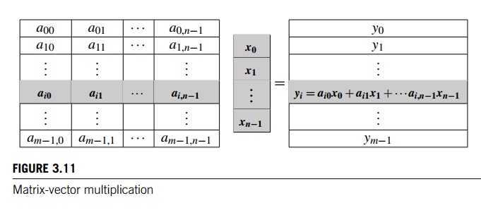
As a final example, let’s look at how we might write an MPI function that multiplies a matrix by a vector. Recall that if A = (a_ij) is an mxn matrix and x is a vector with n components, then y = Ax is a vector with m components and we can find the ith component of y by forming the dot product of the ith row of A with x:

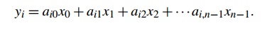
See Figure 3.11.

 

Thus, we might write pseudo-code for serial matrix multiplication as follows:

 

/* For each row of A */

for (i = 0; i < m; i++) {

 

/* Form dot product of ith row with x */

y[i] = 0.0;

 

for (j = 0; j < n; j++)

y[i] += A[i][j] x[j];

}

In fact, this could be actual C code. However, there are some peculiarities in the way that C programs deal with two-dimensional arrays (see Exercise 3.14), so C programmers frequently use one-dimensional arrays to “simulate” two-dimensional arrays. The most common way to do this is to list the rows one after another. For example, the two-dimensional array

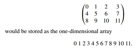
In this example, if we start counting rows and columns from 0, then the element stored in row 2 and column 1 in the two-dimensional array (the 9), is located in position 2 x 4 + 1 = 9 in the one-dimensional array. More generally, if our array has n columns, when we use this scheme, we see that the element stored in row i and column j is located in position I x  n + j in the one-dimensional array. Using this one-dimensional scheme, we get the C function shown in Program 3.11.

 

Now let’s see how we might parallelize this function. An individual task can be the multiplication of an element of A by a component of x and the addition of this product into a component of y. That is, each execution of the statement

 

y[i] += A[i*n+j]*x[j];

 

is a task. So we see that if y[i] is assigned to process q, then it would be convenient to also assign row i of A to process q. This suggests that we partition A by rows. We could partition the rows using a block distribution, a cyclic distribution, or a block-cyclic distribution. In MPI it’s easiest to use a block distribution, so let’s use a block distribution of the rows of A, and, as usual, assume that comm sz evenly divides m, the number of rows.

We are distributing A by rows so that the computation of y[i] will have all of the needed elements of A, so we should distribute y by blocks. That is, if the ith row of A, is assigned to process q, then the ith component of y should also be assigned to process q.

Program 3.11: Serial matrix-vector multiplication

          void Mat_vect_mult(

          double         A[]    /*       in       */,

          double         x[]     /*       in       */,

          double         y[]     /*       out    */,

          int     m       /*       in       */,

          int     n        /*       in       */) {

          int i, j;                                     

          for (i = 0; i < m; i++)      {

          y[i] = 0.0;

          for (j = 0; j < n; j++)

          y[i] += A[i n+j] x[j];

          }

          }  /*  Mat vect mult  */

Now the computation of y[i] involves all the elements in the ith row of A and all the components of x, so we could minimize the amount of communication by simply assigning all of x to each process. However, in actual applications—especially when the matrix is square—it’s often the case that a program using matrix-vector multiplication will execute the multiplication many times and the result vector y from one multiplication will be the input vector x for the next iteration. In practice, then, we usually assume that the distribution for x is the same as the distribution for y.

 

So if x has a block distribution, how can we arrange that each process has access to all the components of x before we execute the following loop?

 

for (j = 0; j < n; j++)

y[i] += A[i][j] x[j];

}

In fact, this could be actual C code. However, there are some peculiarities in the way that C programs deal with two-dimensional arrays (see Exercise 3.14), so C programmers frequently use one-dimensional arrays to “simulate” two-dimensional arrays. The most common way to do this is to list the rows one after another. For example, the two-dimensional array

In this example, if we start counting rows and columns from 0, then the element stored in row 2 and column 1 in the two-dimensional array (the 9), is located in position 2 x 4 + 1 = 9 in the one-dimensional array. More generally, if our array has n columns, when we use this scheme, we see that the element stored in row i and column j is located in position I x  n + j in the one-dimensional array. Using this one-dimensional scheme, we get the C function shown in Program 3.11.

 

Now let’s see how we might parallelize this function. An individual task can be the multiplication of an element of A by a component of x and the addition of this product into a component of y. That is, each execution of the statement

 

y[i] += A[i*n+j]*x[j];

 

is a task. So we see that if y[i] is assigned to process q, then it would be convenient to also assign row i of A to process q. This suggests that we partition A by rows. We could partition the rows using a block distribution, a cyclic distribution, or a block-cyclic distribution. In MPI it’s easiest to use a block distribution, so let’s use a block distribution of the rows of A, and, as usual, assume that comm sz evenly divides m, the number of rows.

We are distributing A by rows so that the computation of y[i] will have all of the needed elements of A, so we should distribute y by blocks. That is, if the ith row of A, is assigned to process q, then the ith component of y should also be assigned to process q.

Program 3.11: Serial matrix-vector multiplication

          void Mat_vect_mult(

          double         A[]    /*       in       */,

          double         x[]     /*       in       */,

          double         y[]     /*       out    */,

          int     m       /*       in       */,

          int     n        /*       in       */) {

          int i, j;                                     

          for (i = 0; i < m; i++)      {

          y[i] = 0.0;

          for (j = 0; j < n; j++)

          y[i] += A[i n+j] x[j];

          }

          }  /*  Mat vect mult  */

Now the computation of y[i] involves all the elements in the ith row of A and all the components of x, so we could minimize the amount of communication by simply assigning all of x to each process. However, in actual applications—especially when the matrix is square—it’s often the case that a program using matrix-vector multiplication will execute the multiplication many times and the result vector y from one multiplication will be the input vector x for the next iteration. In practice, then, we usually assume that the distribution for x is the same as the distribution for y.

 

So if x has a block distribution, how can we arrange that each process has access to all the components of x before we execute the following loop?

 

for (j = 0; j < n; j++)

y[i] += A[i n+j] x[j];

 

Using the collective communications we’re already familiar with, we could execute a call to MPI_Gather followed by a call to MPI_Bcast. This would, in all likelihood, involve two tree-structured communications, and we may be able to do better by using a butterfly. So, once again, MPI provides a single function:

int MPI_Allgather(                 

void* send_buf_p / * in  */,

int     send_count /*       in       */,

MPI_Datatype     send_type   /*       in       */,

Void*          recv_buf_p /*       out    */,

int     recv_count  /*       in       */,

MPI_Datatype     recv_type    /*       in       */,

MPI_Comm         comm          /*       in       */);

This function concatenates the contents of each process’ send_buf_p and stores this in each process’ recv_buf_p. As usual, recv_count is the amount of data being received from each process, so in most cases, recv_count will be the same as send count.

 

Program 3.12: An MPI matrix-vector multiplication function

  

          void Mat_vect_mult(

          double         local_A[]    /         in       /,

          double         local_x[]     /         in       /,

          double         local_y[]     /         out    /,

          int     local_m       /         in       /,

          int     n        /         in       /,

          int     local_n        /         in       /,

          MPI_Comm         comm          /         in       /) f

          double  x;

          int local_i, j;

          int local_ok = 1;

          x = malloc(n sizeof(double));

          MPI_Allgather(local_x, local_n, MPI_DOUBLE,

          x, local_n, MPI_DOUBLE, comm);

          for (local_i = 0; local_i < local_m; local_i++) {

          local_y[local_i] = 0.0;

          for (j = 0; j < n; j++)

          local_y[local_i] += local_A[local_i*n+j]*x[j];

          }

          free(x);

          }  /*  Mat vect mult  */

 

We can now implement our parallel matrix-vector multiplication function as shown in Program 3.12. If this function is called many times, we can improve per-formance by allocating x once in the calling function and passing it as an additional argument.