Boundary Value Problems In Ordinary And Partial Differential Equations

Boundary value Problems in ODE&PDE

BOUNDARY VALUE PROBLEMS IN ODE & PDE

1 Solution of Boundary Value Problems in ODE

2 Solution of Laplace Equation and Poisson Equation

Solution of Laplace Equation – Leibmann`s iteration process

Solution of Poisson Equation

3 Solution of One Dimensional Heat Equation

Bender-Schmidt Method

Crank- Nicholson Method

4 Solution of One Dimensional Wave Equation

1 Solution of Boundary value problems in ODE

Introduction

The solution of a differential equation of second order of the form F (x, y, y’ , y’’ )   0 contains two arbitrary constants. These constants are determined by means of two conditions. The conditions on y and y’or their combination are prescribed at two different values of x are called boundary conditions.

The differential equation together with the boundary conditions is called a boundary value problem.

In this chapter ,we consider the finite difference method of solving linear boundary value problems of the form.

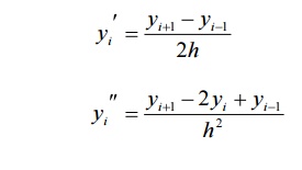
Finite difference approximations to derivatives

First derivative approximations

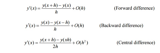
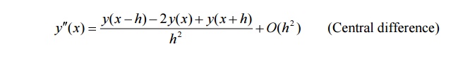
Second derivative approximations

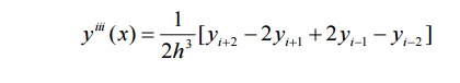
Third derivative approximations

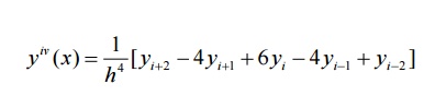
Fourth derivative approximations

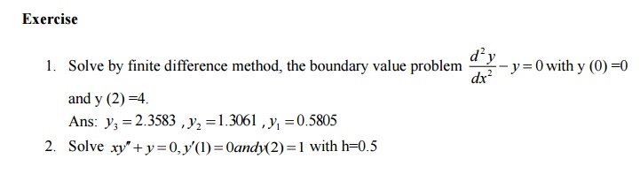
Solution of ordinary differential equations of Second order

Problems

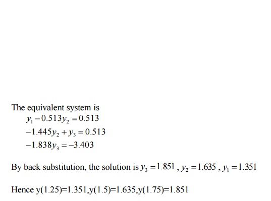
Sol:

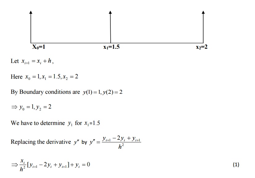
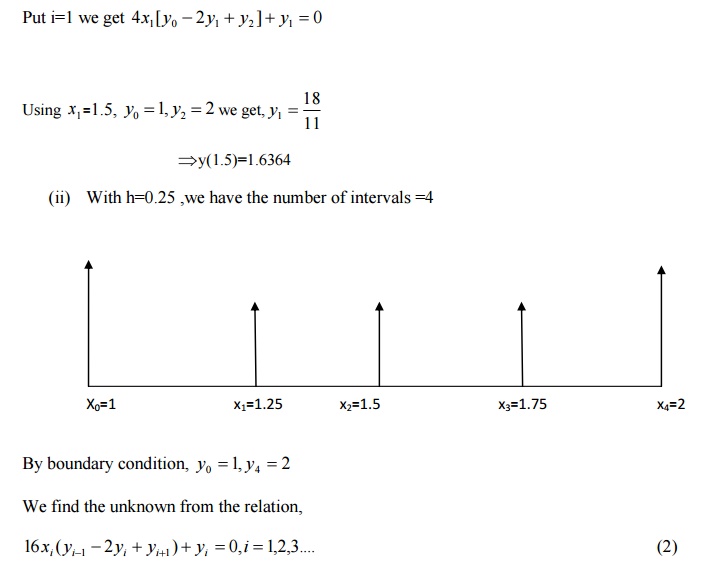
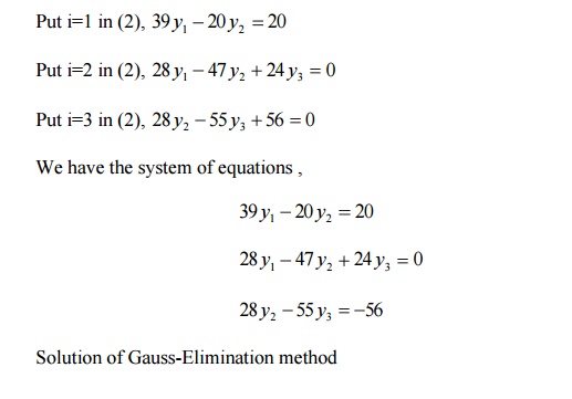
(i)         Divide the interval[1,2] into two sub-intervals with h=(2-1)/2=0.5

2 Solution of Laplace Equation and Poisson equation

Partial differential equations with boundary conditions can be solved in a region by replacing the partial derivative by their finite difference approximations. The finite difference approximations to partial derivatives at a point (x_i,y_i) are given below. The xy-plane is  divided into a network of rectangle of  lengh   ∆x= h and breadth  ∆y=k   by drawing the lines x=ih and y=jk, parallel to x and y axes.The points of intersection of these lines are called grid points or mesh points or lattics points.The grid points ( x_i , y _j ) is denoted by (i,j) and is surrounded by the neighbouring grid points (i-1,j),(i+1,j),(i,j-1),(i,j+1) etc.,

Note

The most general linear P.D.E of second order can be written as

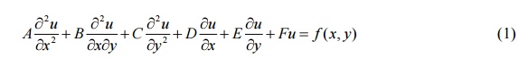
Where A,B,C,D,E,F are in general functions of x and y.

The equation (1) is said to be

Elliptic if B²-4AC<0

Parabolic if B²-4AC=0

Hyperbolic if B²-4AC>0

Solution of Laplace equation u_xx+u_yy=0

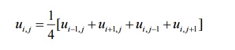
This formula is called Standard five point formula

 This expression is called diagonal five point formula.

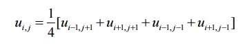
Leibmann’s Iteration   Process

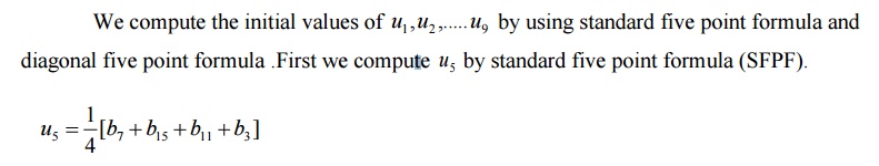
We compute u₁ ,u₃ ,u₇ .u₉  by using diagonal five point formula (DFPF)

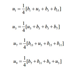
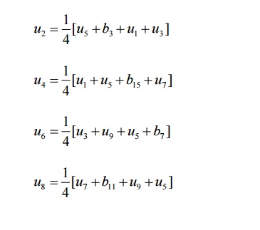
Finally we compute u₂ ,u₄ ,u₆ ,u₈  by using standard five point formula.

The use of Gauss-seidel iteration method to solve the system of equations obtained by finite difference method is called Leibmann’s method.

Problems

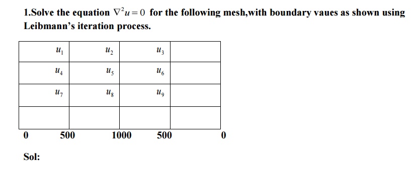
Sol:

Let u₁ , u₂ ……u₉ be the values of u at the interior mesh points of the given region.By symmetry about the lines AB and the line CD,we observe

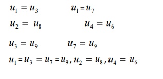
Hence it is enough to find u₁ , u₂ , u₄ , u₅

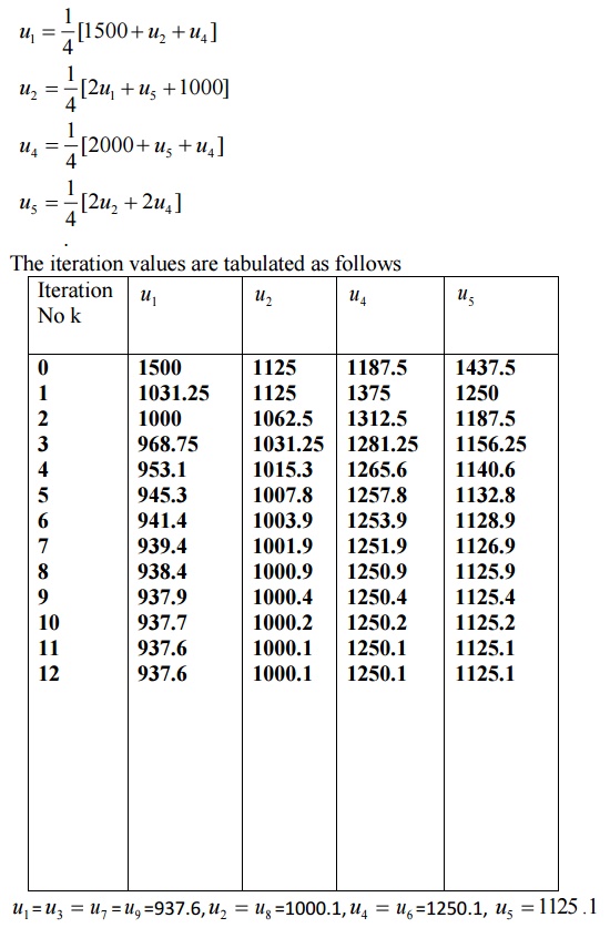
Calculation of rough values

u₅ =1500

u₁ =1125

u₂ =1187.5

u₄ =1437.5

Gauss-seidel scheme

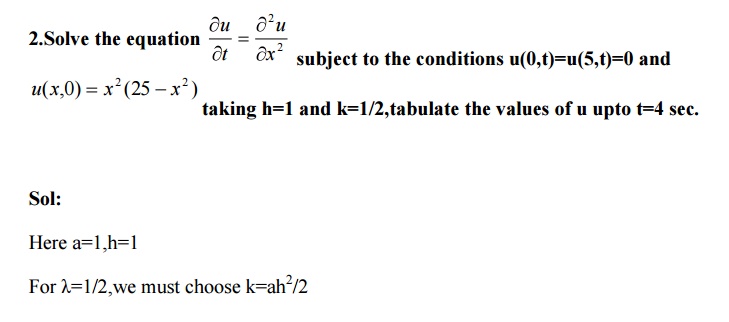
2.When steady state condition prevail,the temperature distribution of the plate is represented by Laplace equation u_xx+u_yy=0.The temperature along the edges of the square plate of side 4 are given by along x=y=0,u=x³ along y=4 and u=16y along x=4,divide the square plate into 16 square meshes of side h=1 ,compute the temperature a iteration process.

Solution of Poisson equation

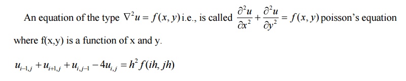
This expression is called the replacement formula.applying this equation at each internal mesh point ,we get a system of linear equations in u_i,where u_i are the values of u at the internal mesh points.Solving the equations,the values u_i are known.

Problems

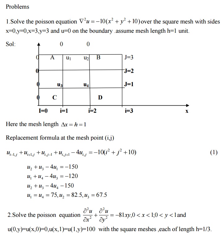
u(0,y)=u(x,0)=0,u(x,1)=u(1,y)=100 with the square meshes ,each of length h=1/3.

3 Solution of One dimensional heat equation

In this session, we will discuss the finite difference solution of one dimensional heat flow equation by Explicit and implicit method

Explicit Method(Bender-Schmidt method

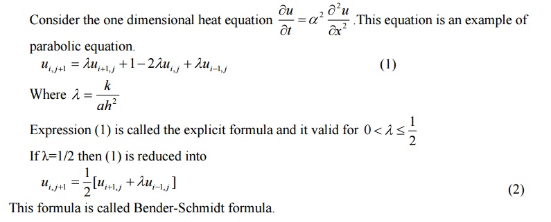
This formula is called Bender-Schmidt formula.

Implicit method (Crank-Nicholson method)

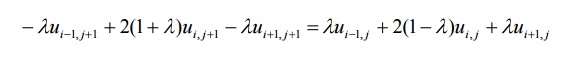
This expression is called Crank-Nicholson’s implicit scheme. 

This expression is called Crank-Nicholson’s implicit scheme. We note that Crank Nicholson’s scheme converges for all values of λ

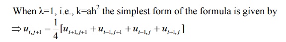
The use of the above simplest scheme is given below.

The value of u at A=Average of the values of u at B, C, D, E

Note

In this scheme, the values of u at a time step are obtained by solving a system of linear equations in the unknowns u_i.

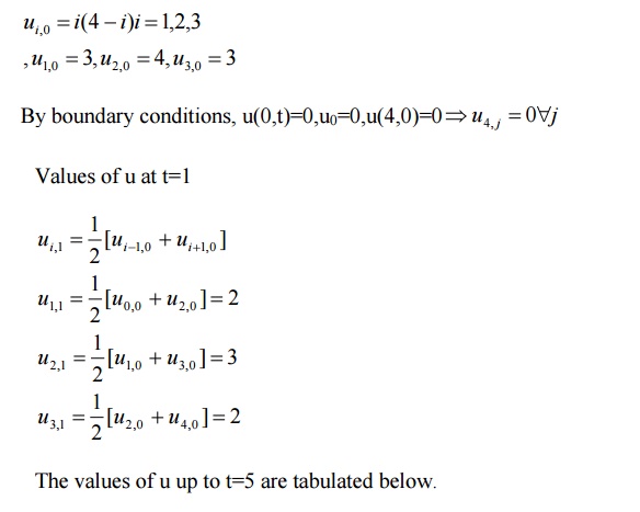
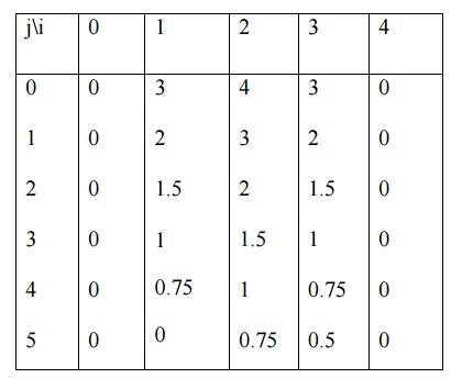
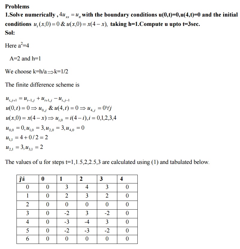
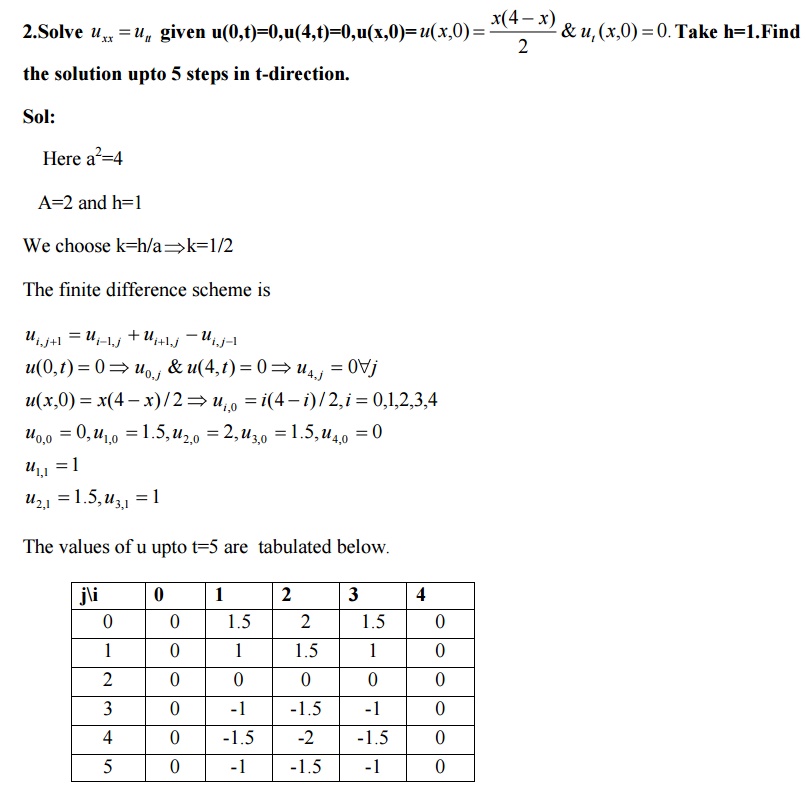
Solved Examples when u(0,t)=0,u(4,t)=0 and with initial condition u(x,0)=x(4-x) upto t=sec

1.Solve u _xx = 2u_t  assuming ∆x=h=1

Sol:

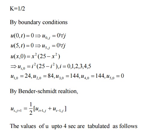
By Bender-Schmidt recurrence relation ,

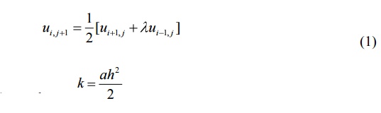
For applying eqn(1) ,we choose

Here a=2,h=1.Then k=1                            

By initial conditions, u(x,0)=x(4-x) ,we have

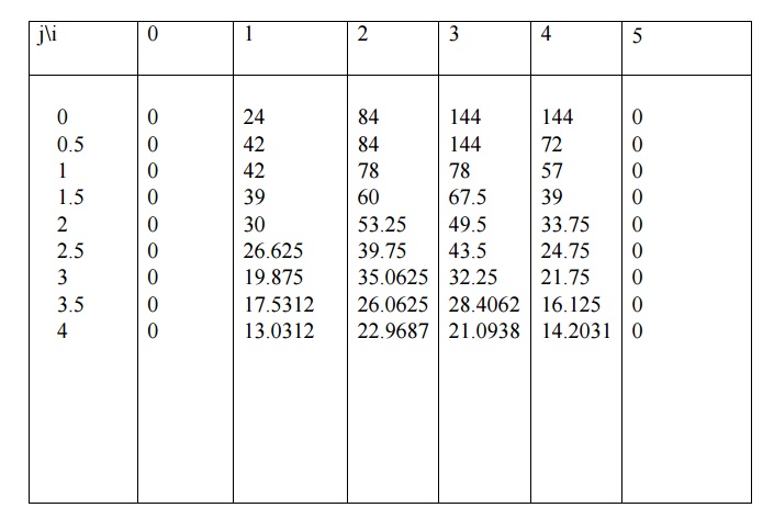
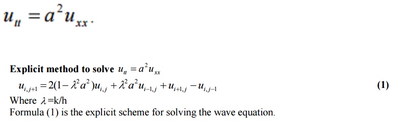
4 Solution of One dimensional wave equation

Introduction

The one dimensional wave equation is of hyperbolic type. In this session, we discuss the finite difference solution of the one dimensional wave equation

Part A

1.What is the error for solving Laplace and Poisson’s equations by finite difference method?

Sol:

The error in replacing by the difference expression is of the order . Since h=k, the error in replaing by the difference expression is of the order .

2. Define a difference quotient.

Sol:

A difference quotient is the quotient obtained by dividing the difference between two values of a function by the difference between two corresponding values of the independent variable.

3. Why is Crank  Nicholson’s scheme called an implicit scheme?

Sol:

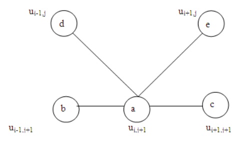
The Schematic representation of crank Nicholson method is shown below.

The solution value at any point (i,j+1) on the (j +1)^th level is dependent on the solution values at the neighboring points on the same level and on three values on the j ^th level. Hence it is an implicit method.

4. What are the methods to solve second order boundary-value problems?

Sol:

(i)Finite difference method (ii)Shooting method.

5. What is the classification of one dimensional heat flow equation.

Sol:

One dimensional heat flow equation is

Here A=1,B=0,C=0

B² −4AC = 0

Hence the one dimensional heat flow equation is parabolic.

6. 6. State Schmidt’s explicit formula for solving heat flow equation

Sol:  ---- ---- 

7.  Write an explicit formula to solve numerically the heat equation (parabolic equation) 

Sol:

--------- ----------

x and k is the space in the time direction).

The above formula is a relation between the function values at the two levels j+1 and j and is called a two level formula. The solution value at any point (i,j+1) on the (j+1)^th level is expressed in terms of the solution values at the points (i-1,j),(i,j) and (i+1,j) on the j th level.Such a method is called explicit formula. the formula is geometrically represented below.

8. State the condition for the equation to be

(i) elliptic,(ii)parabolic(iii)hyperbolic when A,B,C are functions of x and y

Sol:

The equation is elliptic if (2B² ) −4AC < 0

(i.e) B² −AC < 0. It is parabolic if B² −AC = 0 and hyperbolic if B²−4AC > 0

9. Write a note on the stability and convergence of the solution of the difference

equation corresponding to the hyperbolic equation    .

Sol:

For ,λ= the solution of the difference equation is stable and coincides with the solution of the differential equation. For λ> ,the solution is unstable.

For λ<  ,the solution is stable but not convergent.

10.  State the explicit scheme formula for the solution of the wave equation.

Sol:

The formula to solve numerically the wave equation =0 is

The schematic representation is shown below.

The solution value at any point (i,j+1) on the ( j +1)^th level is expressed in terms of solution values on the previous j and (j-1) levels (and not interms of values on the same level).Hence this is an explicit difference formula.