Chapter: Mathematics (maths) : Random Variables
Random Variables
UNIT - I
Random
Variables
1 Introduction
2 Discrete Random Variables
3 Continuous Random Variables
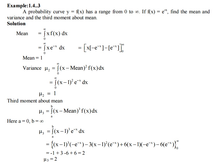
4 Moments
5 Moment generating functions
6 Binomial distribution
7 Poisson distribution
8 Geometric distribution
9 Uniform distribution
10 Exponential distribution
11 Gamma distribution
Introduction
Consider an experiment of throwing a
coin twice. The outcomes {HH, HT, TH, TT} consider the sample space. Each of
these outcome can be associated with a number by specifying a rule of
association with a number by specifying a rule of association (eg. The number
of heads). Such a rule of association is called a random variable. We denote a
random variable by the capital letter (X, Y, etc) and any particular value of
the random variable by x and y.
Thus a random variable X can be
considered as a function that maps all elements in the sample space S into
points on the real line. The notation X(S)=x means that x is the value
associated with the outcomes S by the Random variable X.
1
SAMPLE SPACE
Consider an experiment of throwing a
coin twice. The outcomes S = {HH, HT, TH, TT} constitute the sample space.
2
RANDOM VARIABLE
In this sample space each of these
outcomes can be associated with a number by specifying a rule of association.
Such a rule of association is called a random variables.
Eg : Number of heads
We denote random variable by the
letter (X, Y, etc) and any particular value of the random variable by x or y.
S = {HH, HT, TH, TT} X(S) = {2, 1,
1, 0}
Thus a random X can be the
considered as a fun. That maps all elements in the sample space S into points
on the real line. The notation X(S) = x means that x is the value associated
with outcome s by the R.V.X.
Example
In the experiment of throwing a coin
twice the sample space S is S = {HH,HT,TH,TT}. Let X be a random variable
chosen such that X(S) = x (the number of heads).
Note
Any random variable whose only
possible values are 0 and 1 is called a Bernoulli random variable.
2.1
DISCRETE RANDOM VARIABLE
Definition
: A discrete random variable is a
R.V.X whose possible values consitute finite set of values or countably infinite set of values.
Examples
All the R.V.’s from Example : 1 are
discrete R.V’s
Remark
The meaning of P(X ≤a).
P(X ≤a) is simply the probability of
the set of outcomes ‘S’ in the sample space for which X(s) ≤ a.
Or
P(X≤a) = P{S : X(S) ≤ a}
In the above example : 1 we should
write
P(X ≤ 1) = P(HH, HT, TH) = ¾
Here P(X≤1) = ¾ means the
probability of the R.V.X (the number of heads) is less than or equal to 1 is ¾
.
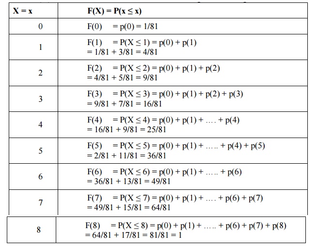
Distribution
function of the random variable X or cumulative distribution of the random
variable X
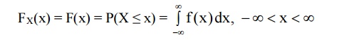
Def
:
The distribution function of a
random variable X defined in (-∞, ∞) is given by F(x) = P(X ≤ x) = P{s : X(s) ≤
x}
Note
Let the random variable X takes
values x1, x2, ….., xn with probabilities P1, P2, ….., Pn and let x1< x2<
….. <xn
Then we have
F(x) =
P(X < x1) = 0, -∞ < x < x,
F(x) =
P(X < x1) = 0, P(X < x1) + P(X = x1) =
0 + p1 = p1
F(x) =
P(X < x2) = 0, P(X < x1) + P(X = x1) + P(X = x2) = p1 + p2
F(x) =
P(X < xn) = P(X < x1) + P(X = x1) + ….. + P(X = xn)
=
p1 + p2+ ………. + pn = 1
2.2
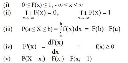
PROPERTIES OF DISTRIBUTION FUNCTIONS
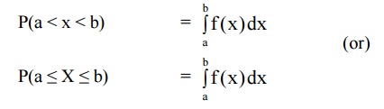
Property : 1 P(a < X ≤ b) =
F(b) – F(a), where F(x) = P(X ≤ x)
Property : 2 P(a ≤ X ≤ b) = P(X =
a) + F(b) – F(a)
Property : 3 P(a < X < b) =
P(a < X ≤ b) - P(X = b)
= F(b) – F(a) – P(X = b) by prob (1)
2.3
PROBABILITY MASS FUNCTION (OR) PROBABILITY FUNCTION
Let X be a one dimenstional discrete R.V. which takes the values x1, x2, …… To each possible outcome
‘xi’ we can associate a number pi.
i.e., P(X = xi) = P(xi) = pi called
the probability of xi. The number pi =
P(xi) satisfies the following conditions.
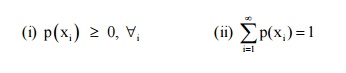
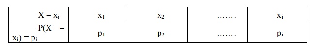
The function p(x) satisfying the
above two conditions is called the probability mass function (or) probability
distribution of the R.V.X. The probability distribution {xi, pi} can be
displayed in the form of table as shown below.
Notation
Let ‘S’ be a sample space. The set of all
outcomes ‘S’ in S such that X(S) = x is denoted by writing X = x.
P(X = x) = P{S : X(s) = x}
|||ly P(x ≤ a) = P{S : X() ∈ (-∞, a)}
and P(a < x ≤ b) = P{s : X(s) ∈ (a, b)}
P(X = a or X = b) = P{(X = a) ∪ (X = b)}
P(X = a and X = b) = P{(X = a) ∩ (X
= b)} and so on.
Theorem
:1 If X1 and X2 are random variable
and K is a constant then KX1, X1 + X2, X1X2,
K1X1 + K2X2, X1-X2
are also random variables.
Theorem
:2
If ‘X’ is a random variable and f(•)
is a continuous function, then f(X) is a random variable.
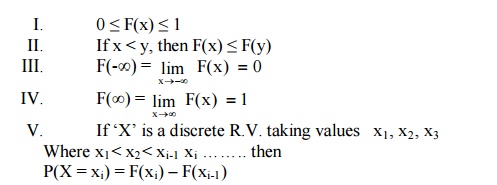
Note
If F(x) is the distribution function
of one dimensional random variable then
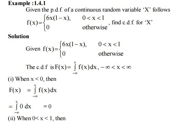
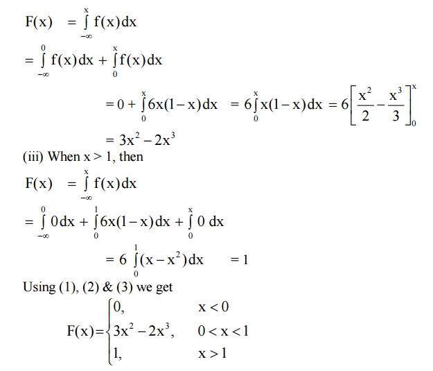
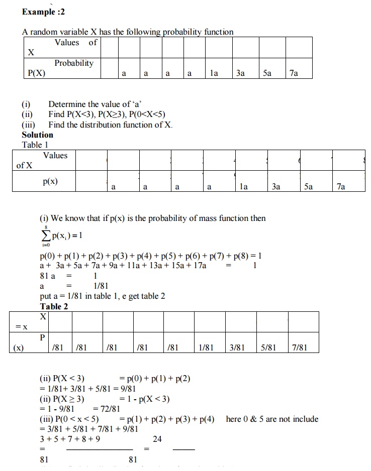
Example:
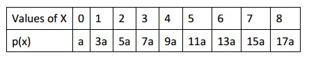
A random variable X has the following
probability function
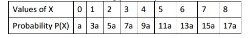
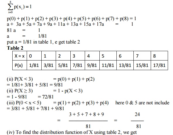
(i) Determine
the value of ‘a’
(ii) Find
P(X<3), P(X≥3), P(0<X<5)
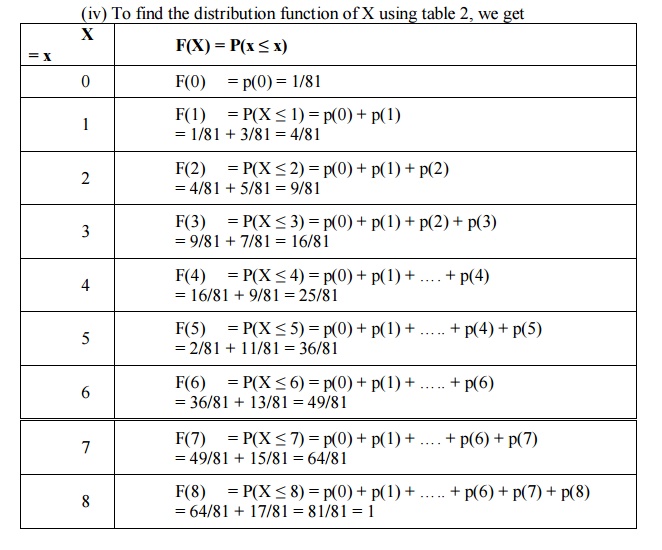
(iii) Find the distribution function of X.
Solution
Table 1
(i)
We
know that if p(x) is the probability of mass function then
3 CONTINUOUS RANDOM VARIABLE
Def : A
R.V.’X’ which takes all possible values in a given internal is called a
continuous random variable.
Example : Age, height, weight are continuous R.V.’s.
3.1 PROBABILITY DENSITY FUNCTION
Consider a continuous R.V. ‘X’
specified on a certain interval (a, b) (which can also be a infinite interval
(-∞, ∞)).
If there is a function y = f(x) such
that
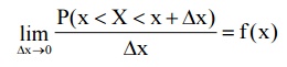
Then this function f(x) is termed as
the probability density function (or) simply density function of the R.V. ‘X’.
It
is also called the frequency function, distribution density or the probability
density function.
The curve y = f(x) is called the
probability curve of the distribution curve.
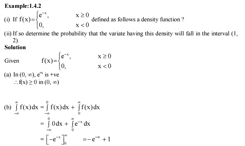
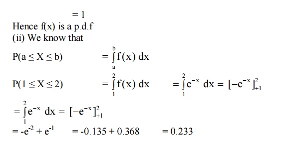
Remark
If f(x) is p.d.f of the R.V.X then
the probability that a value of the R.V. X will fall in some interval (a, b) is
equal to the definite integral of the function f(x) a to b.
3.2 PROPERTIES OF P.D.F
The p.d.f f(x) of a R.V.X has the
following properties
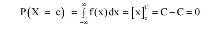
1. In
the case of discrete R.V. the probability at a point say at x = c is not zero.
But in the case of a continuous R.V.X the probability at a point is always
zero.
2. If x is a continuous R.V. then we
have p(a ≤ X ≤ b) = p(a ≤ X < b)
= p(a < X V b)
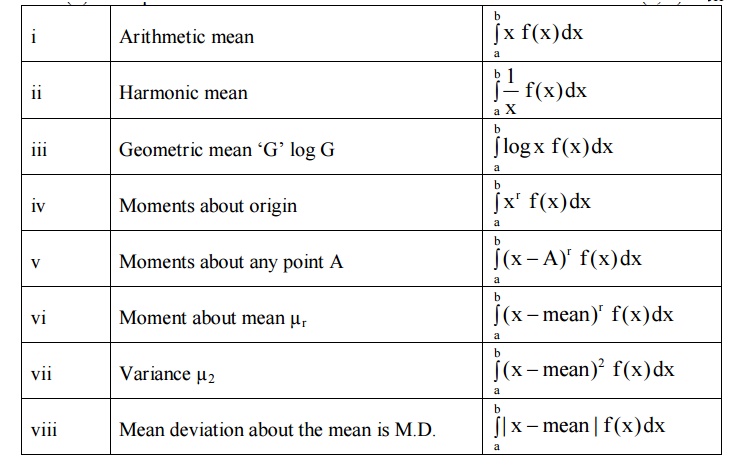
IMPORTANT
DEFINITIONS INTERMS OF P.D.F
If f(x) is the p.d.f of a random
variable ‘X’ which is defined in the interval (a, b) then
3.3
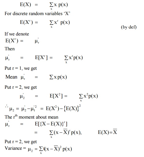
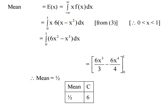
Mathematical Expectations
Def
:Let ‘X’ be a continuous random
variable with probability density function f(x). Then the mathematical expectation of ‘X’ is denoted by E(X) and is
given by

3.4
EXPECTATIONS (Discrete R.V.’s)
Let ‘X’ be a discrete random
variable with P.M.F p(x)
Then
3.5
ADDITION THEOREM (EXPECTATION)
Theorem
1
If X and Y are two continuous random
variable with pdf fx(x) and fy(y) then
E(X+Y) = E(X) + E(Y)
3.6
MULTIPLICATION THEOREM OF EXPECTATION
Theorem
2
If X and Y are independent random
variables,
Then E(XY) = E(X) . E(Y)
Note
:
If X1, X2, ……, Xn are ‘n’
independent random variables, then
E[X1, X2, ……, Xn] = E(X1), E(X2),
……, E(Xn)
Theorem
3
If ‘X’ is a random variable with pdf
f(x) and ‘a’ is a constant, then
(i)
E[a
G(x)] = a E[G(x)]
(ii)
E[G(x)+a]
= E[G(x)+a]
Where G(X) is a function of ‘X’
which is also a random variable.
Theorem
4
If ‘X’ is a random variable with
p.d.f. f(x) and ‘a’ and ‘b’ are constants, then E[ax + b] = a E(X) + b
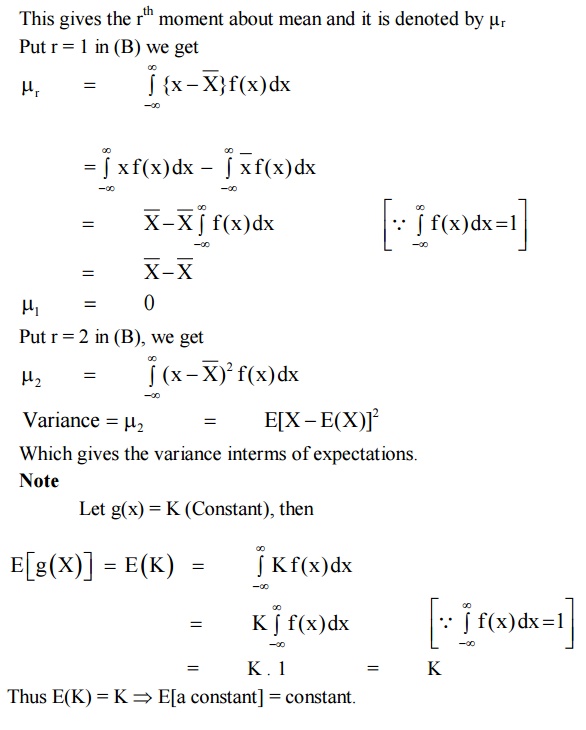
Cor
1:
If we take a = 1 and b = –E(X) = – X
, then we get
![]()
E(X- X ) = E(X) – E(X) = 0
![]()
Note
3.7
EXPECTATION OF A LINEAR COMBINATION OF RANDOM VARIABLES
Let X1, X2,
……, Xn be any ‘n’ random variable and if a1, a2 , ……, an are constants, then
E[a1X1 + a2X2 + ……+ anXn] = a1E(X1) + a2E(X2)+ ……+ anE(Xn)
Result
If X is a random variable, then
Var (aX + b) = a2Var(X)
‘a’ and ‘b’ are constants.
Covariance
:
If
X and Y are random variables, then covariance between them is defined as Cov(X,
Y) = E{[X - E(X)] [Y - E(Y)]}
Cov(X,
Y) = E(XY)
– E(X) . E(Y) (A)
If X and Y are independent, then
E(XY) = E(X) E(Y)
Sub (B) in (A), we get Cov (X, Y) =
0
∴ If X and Y are independent, then
Cov (X, Y) = 0
Note
(i) Cov(aX, bY) = ab Cov(X, Y)
(ii) Cov(X+a, Y+b) = Cov(X, Y)
(iii) Cov(aX+b, cY+d) = ac Cov(X, Y)
(iv) Var (X1 + X2) = Var(X1) + Var(X2) + 2
Cov(X1, X2)
If X1, X2 are independent
Var
(X1+ X2) = Var(X1) + Var(X2)
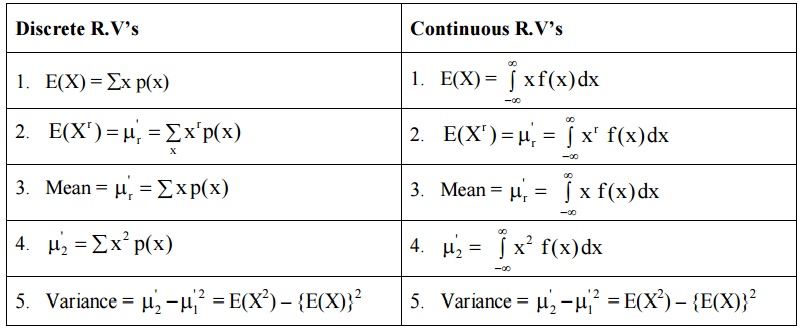
EXPECTATION
TABLE
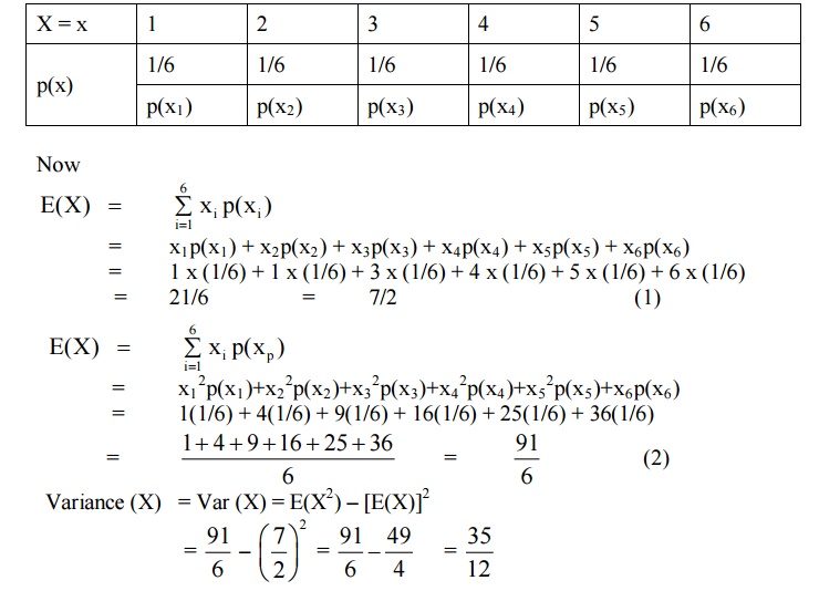
SOLVED PROBLEMS ON DISCRETE R.V’S
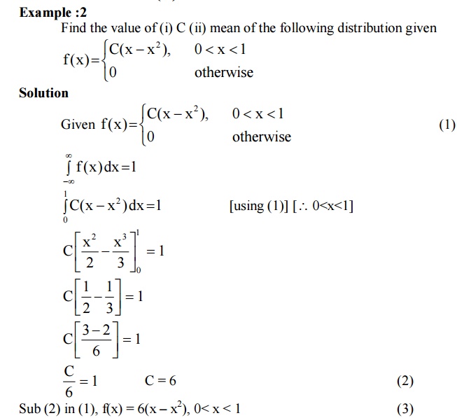
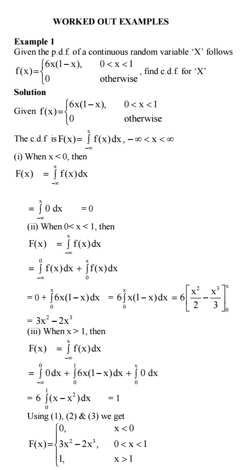
Example :1
When die is thrown, ‘X’ denotes the
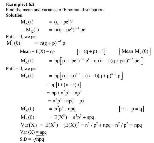
number that turns up. Find E(X), E(X2) and Var (X).
Solution
Let ‘X’ be the R.V. denoting the
number that turns up in a die. ‘X’ takes values 1, 2, 3, 4, 5, 6 and with
probability 1/6 for each
4
CONTINUOUS DISTRIBUTION FUNCTION
Def :
If f(x) is a p.d.f. of a continuous
random variable ‘X’, then the function
is called the distribution function
or cumulative distribution function of the random variable.
*
PROPERTIES OF CDF OF A R.V. ‘X’
5
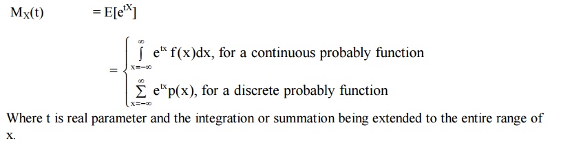
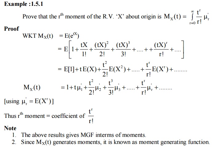
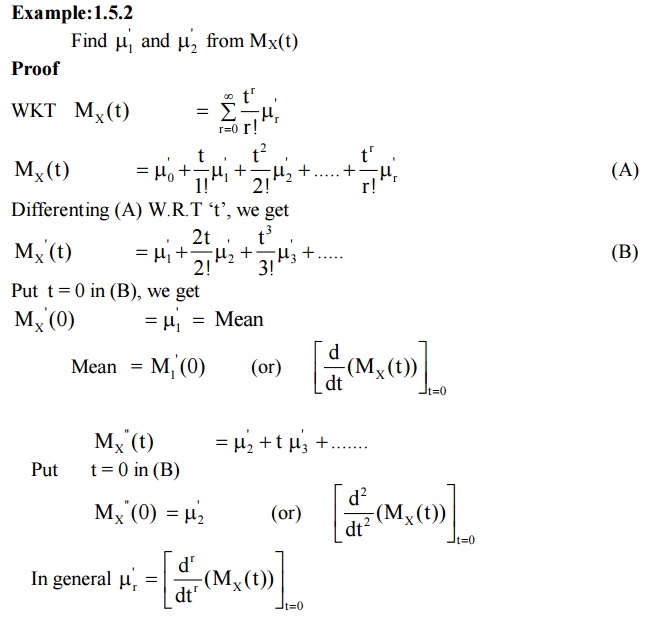
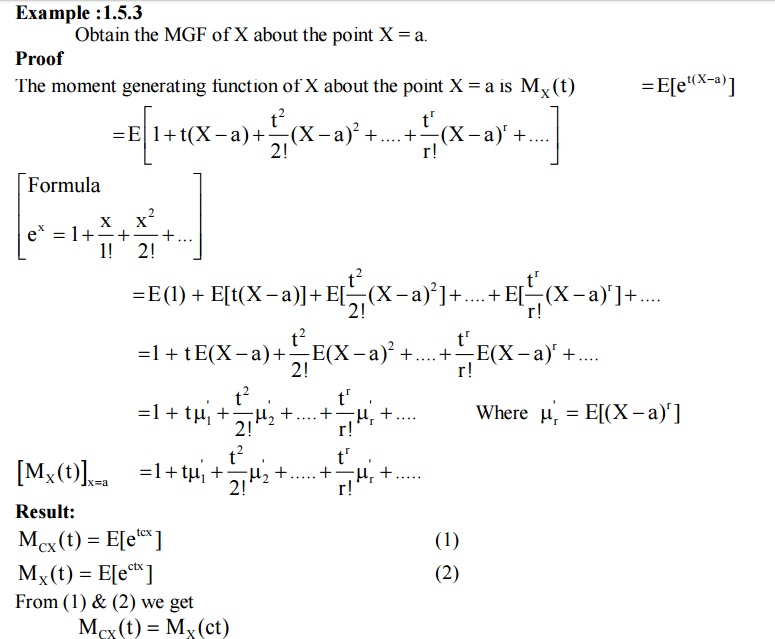
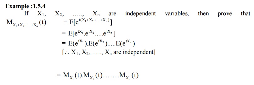
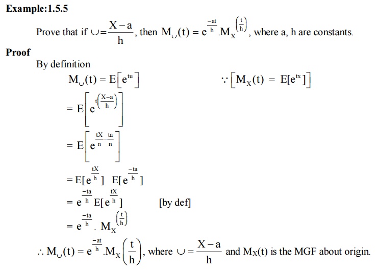
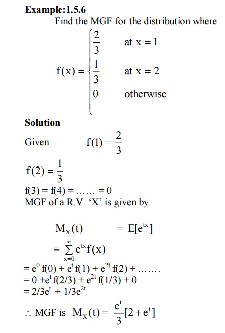
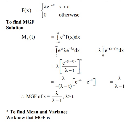
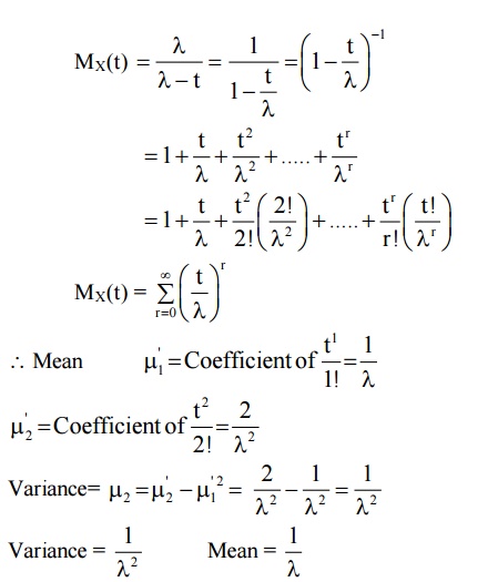
MOMENT GENERATING FUNCTION
Def
: The moment generating function (MGF)
of a random variable ‘X’ (about origin) whose probability function f(x) is given by
6
Discrete Distributions
The important discrete distribution
of a random variable ‘X’ are
1. Binomial Distribution
2. Poisson Distribution
3. Geometric Distribution
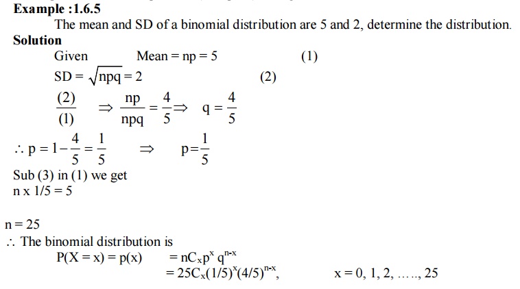
6.1BINOMIAL
DISTRIBUTION
Def
: A random variable X is said to
follow binomial distribution if its probability law is given by
P(x) = p(X = x successes) = nCx px qn-x
Where x = 0, 1, 2, ……., n, p+q = 1
Note
Assumptions in Binomial distribution
i)
There
are only two possible outcomes for each trail (success or failure).
ii) The probability of a success is the
same for each trail.
iii) There are ‘n’ trails, where ‘n’ is a
constant.
iv) The ‘n’ trails are independent.
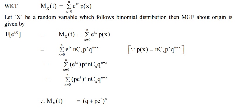
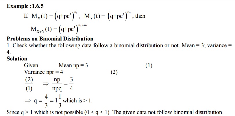
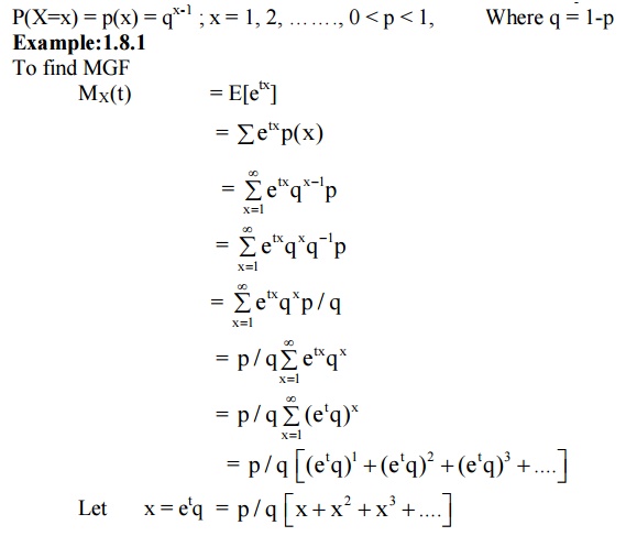
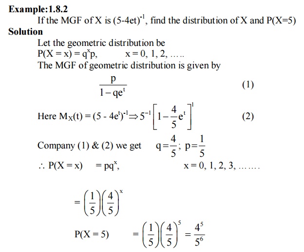
Example
:1.6.1
Find the Moment Generating Function
(MGF) of a binomial distribution about origin.
Solution
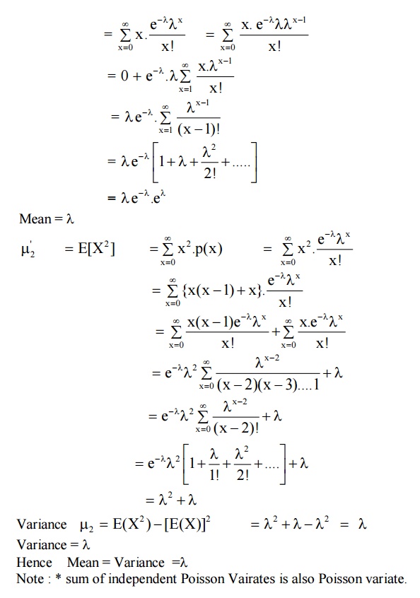
7
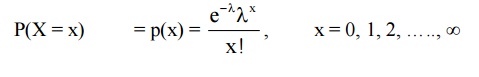
Passion Distribution
Def
:
A random variable X is said to
follow if its probability law is given by
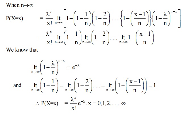
Poisson distribution is a limiting
case of binomial distribution under the following conditions or assumptions.
1. The
number of trails ‘n’ should e infinitely large i.e. n→∞.
2. The
probability of successes ‘p’ for each trail is infinitely small.
3. np
= λ , should be finite where λ is a constant.
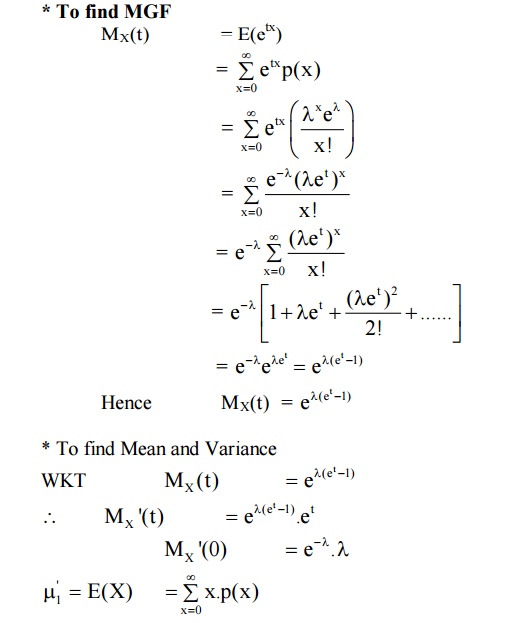
*
To find MGF
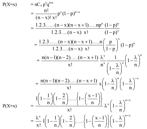
7.3 Derive probability mass function of Poisson distribution as a limiting case of Binomial distribution
Solution
We know that the Binomial
distribution is P(X=x) = nCx pxqn-x
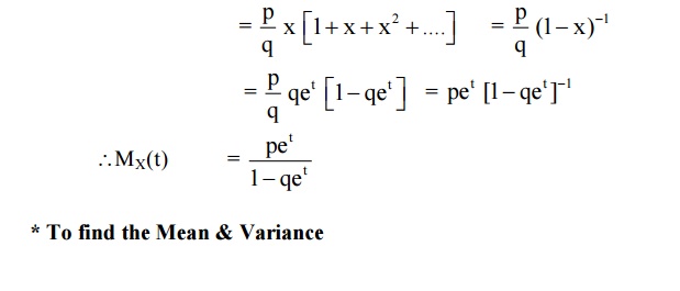
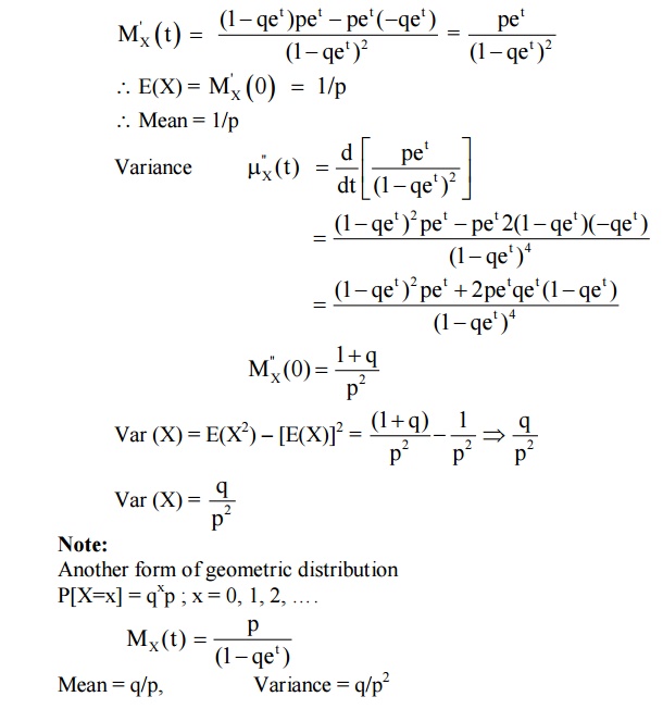
8 GEOMETRIC DISTRIBUTION
Def: A discrete random variable ‘X’ is said to follow geometric distribution, if it assumes only non-negative values and its probability mass function is given by
9 CONTINUOUS DISTRIBUTIONS
If ‘X’ is a continuous random
variable then we have the following distribution
1. Uniform (Rectangular Distribution)
2. Exponential Distribution
3. Gamma Distribution
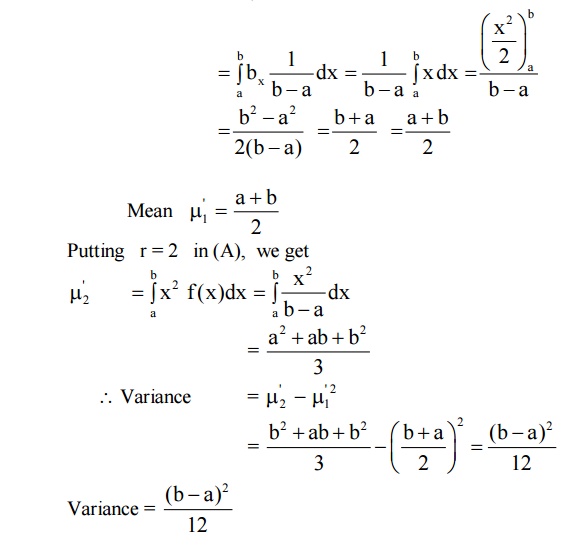
9.1
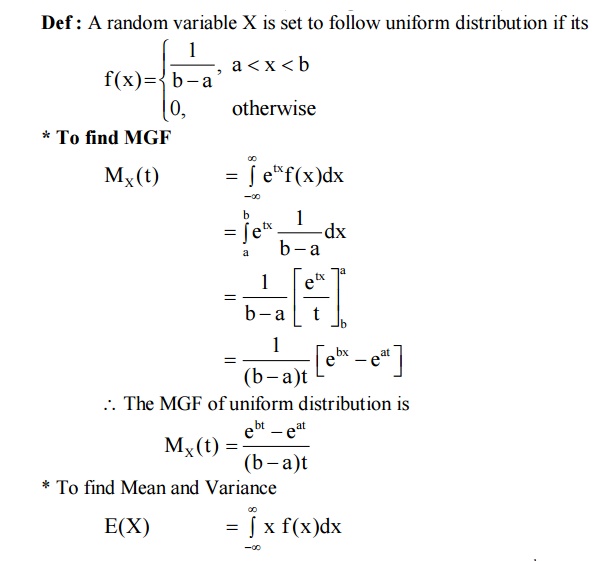
Uniform Distribution (Rectangular Distribution)
Def
: A random variable X is set to follow
uniform distribution if its
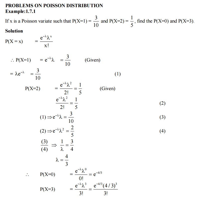
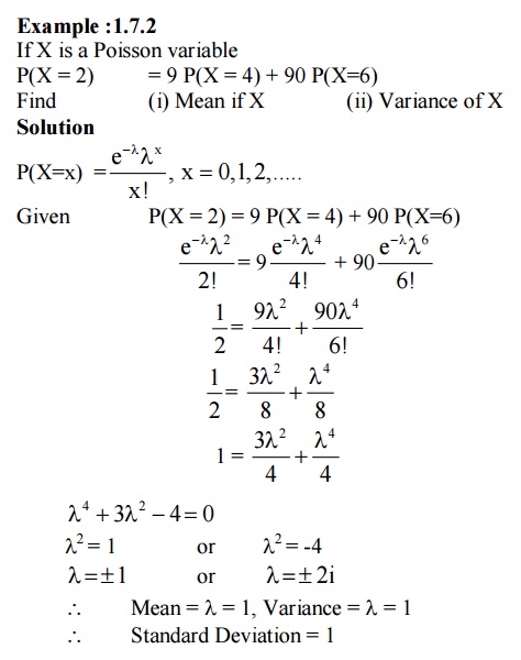
PROBLEMS
ON UNIFORM DISTRIBUTION
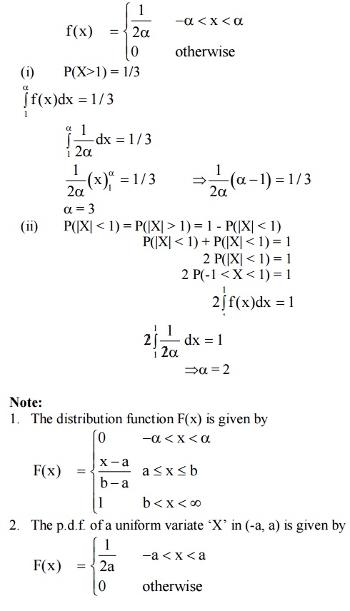
Example
1.9.1
If X is uniformly distributed over
(-α,α), α< 0, find α so that
(i) P(X>1)
= 1/3
(ii) P(|X|
< 1) = P(|X| > 1)
Solution
If X is uniformly distributed in
(-α, α), then its p.d.f. is
10
THE EXPONENTIAL DISTRIBUTION
Def
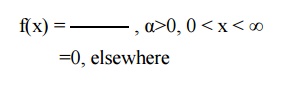
:A continuous random variable ‘X’ is
said to follow an exponential distribution with parameter λ>0 if its probability density
function is given by
11
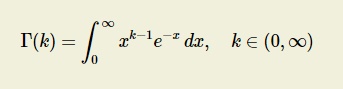
GAMMA DISTRIBUTION
Definition
A Continuous random variable X
taking non-negative values is said to follow gamma distribution , if its
probability density function is given by
When α is the parameter of the
distribution.
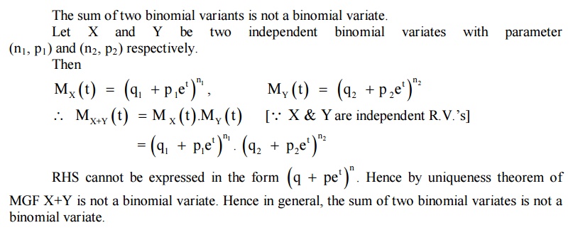
Additive
property of Gamma Variates
If X1,X2 , X3,.... Xk are
independent gamma variates with parameters λ1,λ2,…..λ krespectively then X1+X2
+ X3+.... +Xk is also a gamma variates with parameter λ1+ λ2 +….. + λk
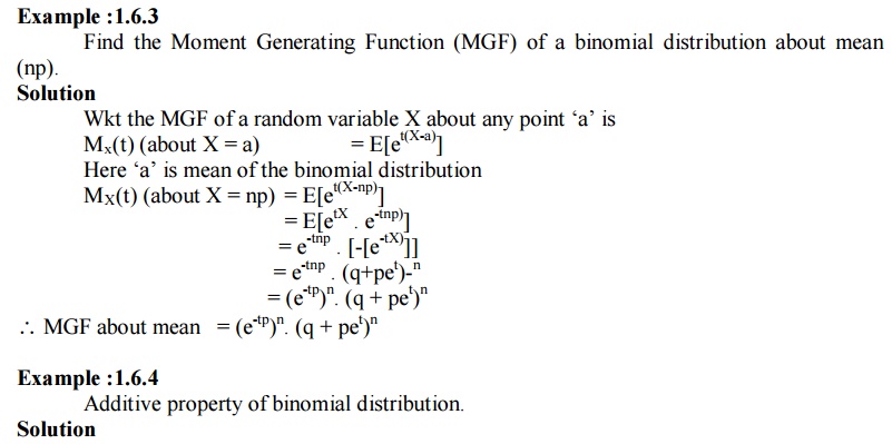
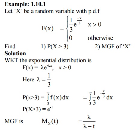
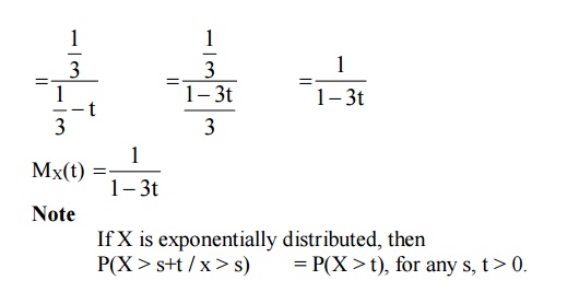
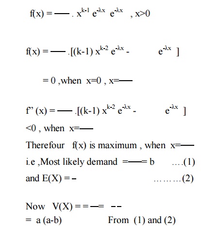
Example
:1.11.1
Customer demand for milk in a
certain locality ,per month , is Known to be a general Gamma RV.If the average
demand is a liters and the most likely demand b liters (b<a) , what is the
varience of the demand?
Solution :
Let X be represent the monthly Customer
demand for milk. Average demand is the value of E(X).
Most likely demand is the value of
the mode of X or the value of X for which its density function is maximum.
If f(x) is the its density function
of X ,then
TUTORIAL
QUESTIONS
1.It is known that the probability
of an item produced by a certain machine will be defective is 0.05. If the
produced items are sent to the market in packets of 20, fine the no. of packets
containing at least, exactly and atmost 2 defective items in a consignment of
1000 packets using (i) Binomial distribution (ii) Poisson approximation to
binomial distribution.
2. The daily consumption of milk in
excess of 20,000 gallons is approximately exponentially distributed with . 3000
= θ The city has a daily stock of 35,000 gallons. What is the probability that
of two days selected at random, the stock is insufficient for both days.
3.The density function of a random
variable X is given by f(x)= KX(2-X), 0≤X≤2.Find K, mean, variance and rth
moment.
4.A binomial variable X satisfies
the relation 9P(X=4)=P(X=2) when n=6. Find the parameter p of the Binomial
distribution.
5. Find
the M.G.F for Poisson Distribution.
6. If
X and Y are independent Poisson variates such that P(X=1)=P(X=2) and
P(Y=2)=P(Y=3). Find V(X-2Y).
7.A discrete random variable has the
following probability distribution
X: 0 1 2 3 4 5 6 7 8
P(X) a 3a 5a 7a 9a 11a 13a 15a 17a
Find the value of a, P(X<3) and
c.d.f of X.
7. In a component manufacturing
industry, there is a small probability of 1/500 for any component to be
defective. The components are supplied in packets of 10. Use Poisson
distribution to calculate the approximate number of packets containing (1). No
defective. (2). Two defective components in a consignment of 10,000 packets.
Related Topics