Polar plot

Polar plot

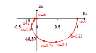
To sketch the polar plot of G(jω) for the entire range of frequency ω, i.e., from 0 to infinity, there are four key points that usually need to be known:

(1) the start of plot where ω = 0,

(2) the end of plot where ω = ∞,

(3) where the plot crosses the real axis, i.e., Im(G(jω)) = 0, and

(4) where the plot crosses the imaginary axis, i.e., Re(G(jω)) = 0.

BASICS OF POLAR PLOT:

o   The polar plot of a sinusoidal transfer function G(jω) is a plot of the magnitude of G(jω) Vs the phase of G(jω) on polar co-ordinates as ω is varied from 0 to ∞.

o   (ie) |G(jω)| Vs angle G(jω) as ω → 0 to ∞.

o   Polar graph sheet has concentric circles and radial lines. Concentric circles represents the magnitude.

o   Radial lines represents the phase angles.

o   In polar sheet

+ve phase angle is measured in ACW from 00 -ve phase angle is measured in CW from 00

PROCEDURE

Express the given expression of OLTF in (1+sT) form.

Substitute s = jω in the expression for G(s)H(s) and get G(jω)H(jω).

Get the expressions for | G(jω)H(jω)| & angle G(jω)H(jω).

Tabulate various values of magnitude and phase angles for different values of ω ranging from 0 to ∞.

Usually the choice of frequencies will be the corner frequency and around corner frequencies.

Choose proper scale for the magnitude circles.

Fix all the points in the polar graph sheet and join the points by a smooth curve.

Write the frequency corresponding to each of the point of the plot.

MINIMUM PHASE SYSTEMS:

Systems with all poles & zeros in the Left half of the s-plane – Minimum Phase Systems.

For Minimum Phase Systems with only poles

Type No. determines at what quadrant the polar plot starts.

Order determines at what quadrant the polar plot ends.

Type No. → No. of poles lying at the origin

Order → Max power of‗s‘ in the denominator polynomial of the transfer function.

GAIN MARGIN

Gain Margin is defined as ―the factor by which the system gain can be increased to drive the system to the verge of instability‖.

For stable systems,

ωgc< ωpc

Magnitude of G(j )H(j ) at ω=ωpc < 1

GM = in positive dB

More positive the GM, more stable is the system.

For marginally stable systems,

ωgc = ωpc

magnitude of G(j )H(j ) at ω=ωpc = 1

GM = 0 dB

For Unstable systems,

ωgc> ωpc

magnitude of G(j )H(j ) at ω=ωpc > 1

GM = in negative dB

Gain is to be reduced to make the system stable

Note:

o   If the gain is high, the GM is low and the system‘s step response shows high overshoots and long settling time.

o   On the contrary, very low gains give high GM and PM, but also causes higher ess, higher values of rise time and settling time and in general give sluggish response.

o   Thus we should keep the gain as high as possible to reduce ess and obtain acceptable response speed and yet maintain adequate GM & PM.

o   An adequate GM of 2 i.e. (6 dB) and a PM of 30 is generally considered good enough as a thumb rule.

t w=w pc , angle of G(jw )H(jw ) = -1800

o   Let magnitude of G(jw)H(jw ) at w = wpc be taken a B

o   If the gain of the system is increased by factor 1/B, then the magnitude of G(jw)H(j w) at w = wpc becomes B(1/B) = 1 and hence the G(jw)H(jw) locus pass through -1+j0 point driving the system to the verge of instability.

o   GM is defined as the reciprocal of the magnitude of the OLTF evaluated at the phase cross over frequency.

GM in dB = 20 log (1/B) = - 20 log B

PHASE MARGIN

Phase Margin is defined as ― the additional phase lag that can be introduced before the system becomes unstable‖.

‘A‘ be the point of intersection of G(j )H(j ) plot and a unit circle centered at the origin. Draw a line connecting the points ‗O‘ & ‗A‘ and measure the phase angle between the line OA and

+ve real axis.

This angle is the phase angle of the system at the gain cross over frequency.

Angle of G(jwgc)H(jw gc) =φ gc

If  an  additional  phase  lag  of  φ  PM  is  introduced  at  this  frequency,  then  the  phase  angle

G(jwgc)H(jw gc) will become 180 and the point ‗A‗ coincides with (-1+j0) driving the system to the verge of instability.

This additional phase lag is known as the Phase Margin.

γ= 1800 + angle of G(jwgc)H(jw gc)

γ= 1800 + φ gc

[Since φ gc is measured in CW direction, it is taken as negative] For a stable system, the phase margin is positive.

A Phase margin close to zero corresponds to highly oscillatory system.

A polar plot may be constructed from experimental data or from a system transfer function

If the values of w are marked along the contour, a polar plot has the same information as a bode plot.

Usually, the shape of a polar plot is of most interest.