Inventory Control

         INVENTORY  CONTROL

Inventory control is concerned with achieving an appropriate compromise between two opposing objectives: (I) minimizing the cost of holding inventory and (2) maximizing service to. customers. On the one hand, minimizing inventory cost suggests keeping inventory to a minimum. In the extreme, zero inventory On the other hand, maximizing customer service Implies keeping large stocks on hand from which the customer can choose and immediately lake possession.

The types of Inventory of greatest interest in PPC arc raw materials, purchased components, in-process inventory (WIP), and finished products. The major costs of holding inventory are (1) investment costs, (2) storage costs, and (3) cost of possible obsolescence or spoilage. The three costs arc referred to collectively as carrying costs or holding costs: Investment cost is usually the largest component; for example, when a company borrows money at a high rate or interest to invest in materials being processed in the factory, but the materials arc months away from being delivered to the customer. Companies can minimize holding costs by minimizing the amount of inventory on hand. However, when inventories are minimized, customer service may suffer. inducing customers to take their business elsewhere. This also has a cost, called the stock-out cost. Most companies want 10 minimize stock-out cost and provide good customer service. Thus. they are caught on the horns of an inventory control dilemma: balancing carrying costs against the cost of poor customer service.

In our introduction to MRP (Section 26.2), we distinguished between two types of demand, independent and dependent. Different inventory control procedures are used for in. dependent and dependent demand items. For dependent demand items, MRP is the most widely implemented technique. For independent demand items, order point inventory systems are commonly used.

        Order Point Inventory  Systems

Order point systems are concerned with two related problems that must be solved when managing inventories of independent demand items: (1) how many units should be ordered? and (2) when should the order be placed? The first problem is often solved using economic order quantity formulas. The second problem can be solved using reorder point methods.

Economic Order Quantitv Formula. The problem of deciding on the most appropriate quantity to order or produce arises when the demand rate for the item is fairly constant, and the rate at which the item is produced is significantly greater than its demand rate. This is the typical make-to-stock situation. The same basic problem occurs with dependent demand items when usage of the item is relatively constant over time due to a steady production rate of the final product with which the item is correlated. 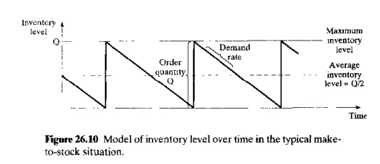In this case, it may make sense to endure some inventory holding costs so that the frequency of setups and their associated costs can be reduced. In these situations where demand rate remains steady, inventory is gradually depleted over time and then quickly replenished to some maximum level determined by the order quantity. The sudden increase and gradual reduction in inventory cause. the inventory level over time to have a saw-tooth appearance, as depicted in Figure 26.10

A total cost equation can be derived for the sum of carrying cost and setup cost for the inventory model in Figure 26.10. Because of the saw-tooth behavior of inventory level, the average inventory level is one-half the maximum level Q in our figure. The total annual inventory cost is therefore given by:

where TIC == total annual inventory cost (holding cost plus ordering cost, $/yr),Q = order quantity (pc/order), Ch = carrying or holding cost ($/pc/yr), C_su = setup cost and/or or

during cost for an order ($/setup or $/order), and D. = annual demand for the item (pc/yr). In the equation, the ratio Da/Q is the number of orders or batches produced per year. which therefore gives the number of setups per year.

The holding cost en consists of two main components, investment cost and storage cost. Both are related to the time that the inventory spends in the warehouse or factory. As previously indicated, the investment eo~1results from the money the company must invest in the inventory before it is sold to customers. This inventory investment cost can be calculated as the interest rate paid by the company i (%/100), multiplied by the value (cost) of the inventory.

Storage cost occurs because the inventory takes up space that must be paid for. The amount of the cost is generally related to the size of the part and how much space it occupies. As an approximation, it can be related to the value or cost of the item stored. For our purposes, this is the most convenient method of valuating the storage cost of an item. By this method, the storage cost equals the cost of the inventory multiplied by the storage rate, ,I'. The term s is the storage cost as a fraction (%/100) of the value of the item in inventory.

Combining interest rate and storage rate into one factor, we have h = i + s. The term h is called the holding cost rate. Like i and s, it is a fraction (%/100) that is multiplied by the cost of the part to evaluate the holding cost of investing in and storing WIP. Accordingly, holding cost can be expressed as follows

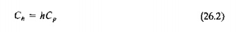
where Ch = holding (carrying) cost ($/pc/yr), Co = unit cost of the item ($/pc). and h = holding cost rate (rate/yr).

Setup cost includes the cost of idle production equipment during the changeover time between batches. The costs of labor performing the setup changes might also be added in. Thus,

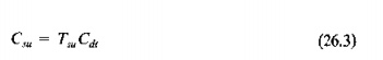
where Csu = setup cost ($/setup or $/order), Tsu = setup or changeover time between batches, (hr /setup or hr/order), and c(dt) = cost rate of machine downtime during the changeover ($/hr). In cases where parts are ordered from an outside vendor, the price quoted by the vendor usually includes a setup cost, either directly or in the form of quantity discounts. Csu should also include the internal costs of placing the order to the vendor.

Eq. (26.1) excludes the actual annual cost of part production. If this cost is included then annual total cost is given by the following equation:

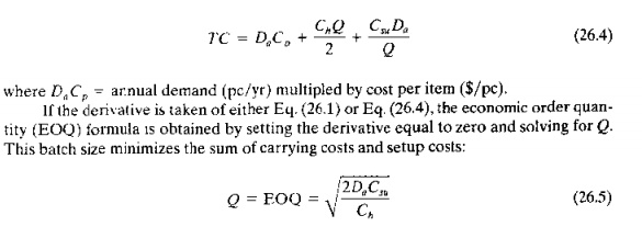
DaDp= arnual demand (pc/yr) multipled by cosst per item (S/pc),

If the derivative is taken of either Eq. (26.1) or Eq. (26.4), the economic order quantity (EOQ) formula IS obtained by setting the derivative equal to zero and solving for Q. This batch size minimizes the sum of carrying costs and setup costs'

where EOQ = economic order quantity (number of parts to be produced per batch, pc/batch or pc/order]. and the other terms have been defined previously.

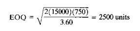
EXAMPLE 26.3  Economic    Order Quantity     Formula

The annual demand for a certain item made-to-stock = 15,000 pc/yr. One unit of the item costs $20.00. and the holding cost rate = 18%/yr. Setup time to produce a batch = 5 hr. The cost of equipment downtime plus labor = $150/hr, Determine the economic order quantity and the total inventory cost for this case.

Solution: Setup cost C,u = 5 x $150 = $750. Holding cost per unit = 0.18 x $20.00 = $3.60. Using these values and the annual demand rate in the EOQ formula, we have

Total inventory cost is given by the TIC equation:

TIC = 0,5(3.60)(2500) + 750(15,000/2500) = $9000

Including the actual production costs in the annual  total, by Eq (26.4) we have:

TC                      =     15J)[)0(20)      + 9000 =  $309,000

The economic order quantity formula has been widely used for determining so-called optimum batch sizes in production. More sophisticated forms of Eqs, (40.1) and (40.4) have appeared in the literature; for example, models that take production rate into account to yield alternative EOQ equations [S]. Eq. 26.5 is the most general form and, in the author's opinion. quite adequate for most real-life situations. The difficulty in applying the EOQ formula is in obtaining accurate values of the parameters in the equation, namely(l) setup cost and (2) inventory carrying costs. These cost factors are usually difficult to evaluate; yet they have an important impact on the calculated economic batch size.

There is no disputing the mathematical accuracy of the EOQ equation. Given specific values of annual demand (D_a),setup cost (C_su).and carrying Cost (e,,), Eq. (26.5) computes  the lowest cost batch size to whatever level of precision the user desires. The trouble is that the user may be lulled into the false belief that no matter how much it CUS1~ to change the setup. the EOO formula always calculates, the optimum batch size. For many years in U.S. industry, this belief tended to encourage lung production runs by manufacturing manager". The thought process went something like this: "If the setup cost increases, we just increase the batch size. because the EOO formula always tells us the optimum production quantity."

The user of the EOQ equation must not lose sight of the total inventory cost ITIC) equation. Eq. (26.1). from which EOQ is derived. Examining the TIC equation. a cost conscious production manager would quickly conclude that both costs and batch sizes can be reduced by decreasing the values of holding cost (c_h) and setup cost (C_us). The production manager may not be able to exert much influence on holding cost because it is determined largely by prevailing interest rates. However. methods can be developed to reduce setup cost by reducing the time required to accomplish the changeover of a machine. Reducing setup times is an important focus in just-in-time review the approaches for reducing setup time in Section 26.7.2

Reorder Point Systems. Determining the economic order quantity is nut the only problem that must be solved in controlling inventories in make-to-stock situations, The

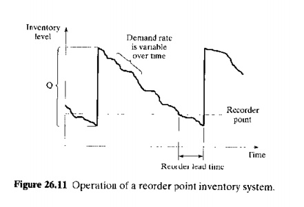
other problem is deciding when to reorder. One of the most widely used methods is the reorder point system. Although we have drawn the inventory level in Figure 26.10 as a very deterministic saw-tooth diagram, the reality is Ihat there are usually variations in demand rate during the inventory order cycle. as illustrated in Figure 26.11. Accordingly, the timing of when to reorder cannot be predicted with the precision that would exist if demand rate were a known constant value. In a reorder point system. when the inventory level for a given stock item falls to some point specified as the reorder point, then an order is placed to restock the item. The reorder point is specified at a sufficient quantity level 10 minimize the probability of a stock-out between when the reorder point is reached and the new order is received. Reorder point triggers can be implemented using computerized inventory control systems that continuously monitor the inventory level as demand occurs and automatically generate an order for a new batch when the level declines below the reorder point

            Work-in-Process   Inventory  Costs

Work-in-process (WIP) represents a significant inventory cost for many manufacturing firms. In effect, the company is continually investing in raw materials, processing those materials, and then delivering them to customers when processing has been completed The problem is that processing takes time, and the company pays a holding cost between start of production and receipt of payment from the customer for goods delivered. In Chapter 2, we showed that WIP and manufacturing lead time (MLT) are closely related. The longer the manufacturing lead time, the greater the WIP. In this section, a method for evaluating the cost of WIP and MLT is presented. The method is based on concepts suggested by Meyer.

In Chapter 2, we indicated that production typically consists of a series of separate manufacturing steps or operations. Time is consumed in each operation, and that time has an associated cost. There is also a time between each operation (at least for most manufacturing situations) that we have referred to as the non-operation time. The non-operation lime includes material handling, inspection. and storage. There is also a cost associated with the non-operation time. These times and costs for a given part can be graphically illustrated as shown in Figure 26.12.At time t == 0, the cost of the part is simply its material cost em' The cost of each processing step on the part is the production time multiplied by the rate for the machine and labor. Production time T_p is determined from Eq. (2.10) and accounts for both setup time and operation time. Let us symbolize the fate as Co'  Non-operation costs (c.g., inspection and material handling) related to the processing step are symbolized by the term C_no Accordingly, the cost associated with each processing step in the manufacturing sequence is the sum

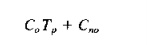
The cost for each step is shown in Figure 26.12 as a vertical line, suggesting no time lapse. This is a simplification in the graph, justified by the fact that the time between operations

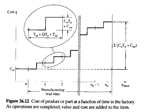
spent waiting and in storage is generally much greater than the tune for processing, handling and inspection

The total cost that has been invested In the part at the end of all operations is the sum of the material cost and the accumulated processing, inspection, and handling costs. Syrnbolizing this part cost as C_p' we can evaluate it using the following equation:

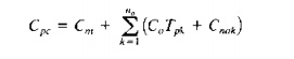
where k is used to indicate the sequence of operations, and there are a lotal of flo operations. For convenience. if we assume that 1~ and Cooare equal for all n., operations, then

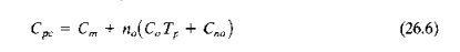
The part cost function shown in Figure 26.12 and represented by Eq. (26.6) can be approximated by a straight line as shown in Figure 26.13. The line starts at lime t = 0 with a value = em and slopes upward 10 the right so that its final value is the same as the final part cost in Figure 26.12. The approximation becomes more accurate as the number of processing steps increases. The equation for this line is

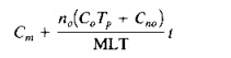
where  MLT =  manufacturing lead time for the part, and t =  time in Figure  26.13.

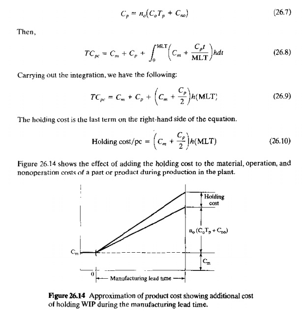
As in our derivation of the economic order quantity formula, we apply the holding cost rate h to the accumulated part cost defined by Eq. (26.6), but substituting the straightline approximation in place of the stepwise cost accumulation in Figure 26.12. In this way, we have an equation for total cost per part that includes the WIP carrying costs:

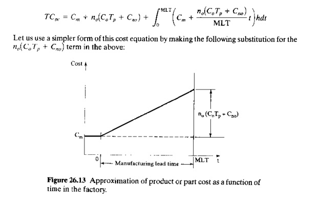
Let us use a simpler form of this cost equation by making the following substitution for the n_o(C_oT_p+C_no) term in the above:

EXAMPLE          26.4   Inventory Holding  Cost for WIP During Manufacturing

The cost of the raw material for a certain part is $100. The part is processed through 20 processing steps in the plant, and the manufacturing lead time is 15 wk. The production time per processing step is 0.8 hr, and the machine and labor rate is $25.00/hr. Inspection, material handling, and other related costs average to $l1Oper processing step by the time the part is finished. The interest rate used by the company i =20%, and the storage rate s = 13%. Determine the cost per part and the holding cost.

The $38.08 in our example  is more than 5% of the cost of the part; yet the holding cost is usually  not included  directly  in the company's  evaluation  of part cost. Rather,  it is considered  as overhead.  Suppose  that  this is a typical  part for the company,  and 5000 similar parts  are processed  through  the plant each year; then the annual  inventory  cost for WIP of 5000 parts  =  5000 x $38.08  ==  $190,400. If the manufacturing   lead time could be reduced to half its current  value, this would translate  into a 50% savings in WIP  holding  cost.