Filter fundamentals, Design of filters

Filter fundamentals, Design of filters

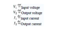
A two-port network (a kind of four-terminal network or quadripole) is an electrical circuit or device with two pairs of terminals connected together internally by an electrical network. Two terminals constitute a port if they satisfy the essential requirement known as the port condition: the same current must enter and leave a port. Examples include small-signal models for transistors (such as the hybrid-pi model), filters and matching networks. The analysis of passive two-port networks is an outgrowth of reciprocity theorems first derived by Lorentz[3].

A two-port network makes possible the isolation of either a complete circuit or part of it and replacing it by its characteristic parameters. Once this is done, the isolated part of the circuit becomes a "black box" with a set of distinctive properties, enabling us to abstract away its specific physical buildup, thus simplifying analysis. Any linear circuit with four terminals can be transformed into a two-port network provided that it does not contain an independent source and satisfies the port conditions. There are a number of alternative sets of parameters that can be used to describe a linear two-port network, the usual sets are respectively called z, y, h, g, and ABCD parameters, each described individually below. These are all limited to linear networks since an underlying assumption of their derivation is that any given circuit condition is a linear superposition of various short-circuit and open circuit conditions. They are usually expressed in matrix notation, and they establish relations between the variables

These current and voltage variables are most useful at low-to-moderate frequencies. At high frequencies (e.g., microwave frequencies), the use of power and energy variables is more appropriate, and the two-port current–voltage approach is replaced by an approach based upon scattering parameters.

The terms four-terminal network and quadripole (not to be confused with quadrupole) are also used, the latter particularly in more mathematical treatments although the term is becoming archaic. However, a pair of terminals can be called a port only if the current entering one terminal is equal to the current leaving the other; this definition is called the port condition. A four-terminal network can only be properly called a two-port when the terminals are connected to the external circuitry in two pairs both meeting the port condition.

Propagation constant

The propagation constant of an electromagnetic wave is a measure of the change undergone by the amplitude of the wave as it propagates in a given direction. The quantity being measured can be the voltage or current in a circuit or a field vector such as electric field strength or flux density. The propagation constant itself measures change per metre but is otherwise dimensionless.

The propagation constant is expressed logarithmically, almost universally to the base e, rather than the more usual base 10 used in telecommunications in other situations. The quantity measured, such as voltage, is expressed as a sinusiodal phasor. The phase of the sinusoid varies with distance which results in the propagation constant being a complex number, the imaginary part being caused by the phase change.

The term propagation constant is somewhat of a misnomer as it usually varies strongly with ω. It is probably the most widely used term but there are a large variety of alternative names used by various authors for this quantity. These include, transmission parameter, transmission function, propagation parameter, propagation coefficient and transmission constant. In plural, it is usually implied that α and β are being referenced separately but collectively as in transmission parameters, propagation parameters, propagation coefficients, transmission constants and secondary coefficients. This last occurs in transmission line theory, the term secondary being used to contrast to the primary line coefficients. The primary coefficients being the physical properties of the line; R,C,L and G, from which the secondary coefficients may be derived using the telegrapher's equation. Note that, at least in the field of transmission lines, the term transmission coefficient has a different meaning despite the similarity of name. Here it is the corollary of reflection coefficient.

The propagation constant, symbol γ, for a given system is defined by the ratio of the amplitude at the source of the wave to the amplitude at some distance x, such that,

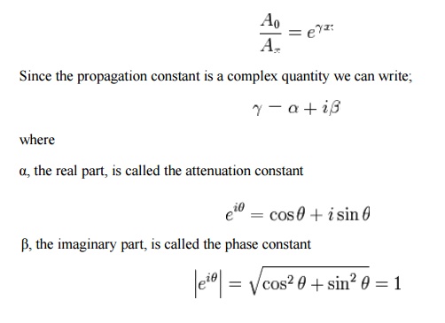
That β does indeed represent phase can be seen from Euler's formula; which is a sinusoid which varies in phase as θ varies but does not vary in amplitude because; The reason for the use of base e is also now made clear. The imaginary phase constant, iβ, can be added directly to the attenuation constant, α, to form a single complex number that can be handled in one mathematical operation provided they are to the same base. Angles measured in radians require base e, so the attenuation is likewise in base e.

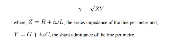
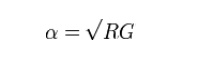
For a copper transmission line, the propagation constant can be calculated from the primary line coefficients by means of the relationship;

Attenuation constant

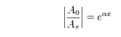
In telecommunications, the term attenuation constant, also called attenuation parameter or coefficient, is the attenuation of an electromagnetic wave propagating through a medium per unit distance from the source. It is the real part of the propagation constant and is measured in nepers per metre. A neper is approximately 8.7dB. Attenuation constant can be defined by the amplitude ratio;

The propagation constant per unit length is defined as the natural logarithmic of ratio of the sending end current or voltage to the receiving end current or voltage.

Copper lines

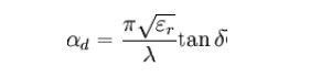
The attenuation constant for copper (or any other conductor) lines can be calculated from the primary line coefficients as shown above. For a line meeting the distortionless condition, with a conductance G in the insulator, the attenuation constant is given by;

however, a real line is unlikely to meet this condition without the addition of loading coils and, furthermore, there are some decidedly non-linear effects operating on the primary "constants" which cause a frequency dependence of the loss. There are two main components to these losses, the metal loss and the dielectric loss.

The loss of most transmission lines are dominated by the metal loss, which causes a frequency dependency due to finite conductivity of metals, and the skin effect inside a conductor. The skin effect causes R along the conductor to be approximately dependent on frequency according to;

Losses in the dielectric depend on the loss tangent (tanδ) of the material, which depends inversely on the wavelength of the signal and is directly proportional to the frequency.

Optical fibre

The attenuation constant for a particular propagation mode in an optical fiber, the real part of the axial propagation constant.

Phase constant

In electromagnetic theory, the phase constant, also called phase change constant, parameter or coefficient is the imaginary component of the propagation constant for a plane wave. It represents the change in phase per metre along the path travelled by the wave at any instant and is equal to the angular wavenumber of the wave. It is represented by the symbol β and is measured in units of radians per metre.

From the definition of angular wavenumber;

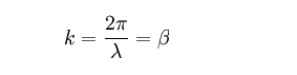
This quantity is often (strictly speaking incorrectly) abbreviated to wavenumber. Properly, wavenumber is given by Y = 1/lamda, which differs from angular wavenumber only by a constant multiple of 2π, in the same way that angular frequency differs from frequency.

For a transmission line, the Heaviside condition of the telegrapher's equation tells us that the wavenumber must be proportional to frequency for the transmission of the wave to be undistorted in the time domain. This includes, but is not limited to, the ideal case of a lossless line. The reason for this condition can be seen by considering that a useful signal is composed of many different wavelengths in the frequency domain. For there to be no distortion of the waveform, all these waves must travel at the same velocity so that they arrive at the far end of the line at the same time as a group. Since wave phase velocity is given by;

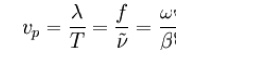
it is proved that β is required to be proportional to ω. In terms of primary coefficients of the line, this yields from the telegrapher's equation for a distortionless line the condition;

However, practical lines can only be expected to approximately meet this condition over a limited frequency band.

Filters

The term propagation constant or propagation function is applied to filters and other two-port networks used for signal processing. In these cases, however, the attenuation and phase coefficients are expressed in terms of nepers and radians per network section rather than per metre. Some authors make a distinction between per metre measures (for which "constant" is used) and per section measures (for which "function" is used).

The propagation constant is a useful concept in filter design which invariably uses a cascaded section topology. In a cascaded topology, the propagation constant, attenuation constant and phase constant of individual sections may be simply added to find the total propagation constant etc.

Cascaded networks:

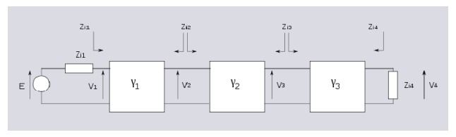
Three networks with arbitrary propagation constants and impedances connected in cascade. The Zi terms represent image impedance and it is assumed that connections are between matching image impedances.

The ratio of output to input voltage for each network is given by,

The terms are impedance scaling terms[3] and their use is explained in the image impedance article.

The overall voltage ratio is given by

Thus for n cascaded sections all having matching impedances facing each other, the overall propagation constant is given by,