Characterizing Schedules Based on Serializability

Characterizing Schedules Based on Serializability

In the previous section, we characterized schedules based on their recoverability properties. Now we characterize the types of schedules that are always considered to be correct when concurrent transactions are executing. Such schedules are known as serializable schedules. Suppose that two users—for example, two airline reservations agents—submit to the DBMS transactions T₁ and T₂ in Figure 21.2 at approxi-mately the same time. If no interleaving of operations is permitted, there are only two possible outcomes:

Execute all the operations of transaction T₁ (in sequence) followed by all the operations of transaction T₂ (in sequence).

Execute all the operations of transaction T₂ (in sequence) followed by all the operations of transaction T₁ (in sequence).

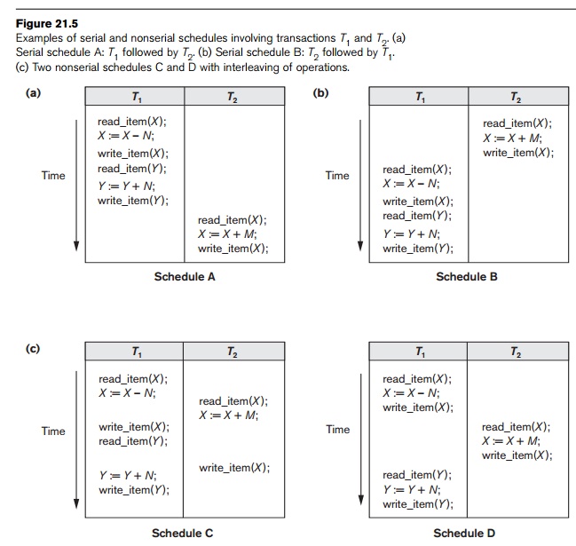
These two schedules—called serial schedules—are shown in Figure 21.5(a) and (b), respectively. If interleaving of operations is allowed, there will be many possible orders in which the system can execute the individual operations of the transactions. Two possible schedules are shown in Figure 21.5(c). The concept of serializability of schedules is used to identify which schedules are correct when transaction executions have interleaving of their operations in the schedules. This section defines serializability and discusses how it may be used in practice.

1. Serial, Nonserial, and Conflict-Serializable Schedules

Schedules A and B in Figure 21.5(a) and (b) are called serial because the operations of each transaction are executed consecutively, without any interleaved operations from the other transaction. In a serial schedule, entire transactions are performed in serial order: T₁ and then T₂ in Figure 21.5(a), and T₂ and then T₁ in Figure 21.5(b). Schedules C and D in Figure 21.5(c) are called nonserial because each sequence interleaves operations from the two transactions.

Formally, a schedule S is serial if, for every transaction T participating in the schedule, all the operations of T are executed consecutively in the schedule; otherwise, the schedule is called nonserial. Therefore, in a serial schedule, only one transaction at a time is active—the commit (or abort) of the active transaction initiates execution of the next transaction. No interleaving occurs in a serial schedule. One reasonable assumption we can make, if we consider the transactions to be independent, is that every serial schedule is considered correct. We can assume this because every transaction is assumed to be correct if executed on its own . Hence, it does not matter which transaction is executed first. As long as every transaction is executed from beginning to end in isolation from the operations of other transactions, we get a correct end result on the database.

The problem with serial schedules is that they limit concurrency by prohibiting interleaving of operations. In a serial schedule, if a transaction waits for an I/O operation to complete, we cannot switch the CPU processor to another transaction, thus wasting valuable CPU processing time. Additionally, if some transaction T is quite long, the other transactions must wait for T to complete all its operations before starting. Hence, serial schedules are considered unacceptable in practice. However, if we can determine which other schedules are equivalent to a serial sched-ule, we can allow these schedules to occur.

To illustrate our discussion, consider the schedules in Figure 21.5, and assume that the initial values of database items are X = 90 and Y = 90 and that N = 3 and M = 2. After executing transactions T₁ and T₂, we would expect the database values to be X = 89 and Y = 93, according to the meaning of the transactions. Sure enough, executing either of the serial schedules A or B gives the correct results. Now consider the nonserial schedules C and D. Schedule C (which is the same as Figure 21.3(a)) gives the results X = 92 and Y = 93, in which the X value is erroneous, whereas schedule D gives the correct results.

Schedule C gives an erroneous result because of the lost update problem discussed in Section 3; transaction T₂ reads the value of X before it is changed by transaction T₁, so only the effect of T₂ on X is reflected in the database. The effect of T₁ on X is lost, overwritten by T₂, leading to the incorrect result for item X. However, some nonserial schedules give the correct expected result, such as schedule D. We would like to determine which of the nonserial schedules always give a correct result and which may give erroneous results. The concept used to characterize schedules in this manner is that of serializability of a schedule.

The definition of serializable schedule is as follows: A schedule S of n transactions is serializable if it is equivalent to some serial schedule of the same n transactions. We will define the concept of equivalence of schedules shortly. Notice that there are n! possible serial schedules of n transactions and many more possible nonserial schedules. We can form two disjoint groups of the nonserial schedules—those that are equivalent to one (or more) of the serial schedules and hence are serializable, and those that are not equivalent to any serial schedule and hence are not serializable.

Saying that a nonserial schedule S is serializable is equivalent to saying that it is cor-rect, because it is equivalent to a serial schedule, which is considered correct. The remaining question is: When are two schedules considered equivalent?

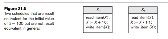
There are several ways to define schedule equivalence. The simplest but least satisfactory definition involves comparing the effects of the schedules on the database. Two schedules are called result equivalent if they produce the same final state of the database. However, two different schedules may accidentally produce the same final state. For example, in Figure 21.6, schedules S₁ and S₂ will produce the same final database state if they execute on a database with an initial value of X = 100; however, for other initial values of X, the schedules are not result equivalent. Additionally, these schedules execute different transactions, so they definitely should not be considered equivalent. Hence, result equivalence alone cannot be used to define equivalence of schedules. The safest and most general approach to defining schedule equivalence is not to make any assumptions about the types of operations included in the transactions. For two schedules to be equivalent, the operations applied to each data item affected by the schedules should be applied to that item in both schedules in the same order. Two definitions of equivalence of schedules are generally used: conflict equivalence and view equivalence. We discuss conflict equivalence next, which is the more commonly used definition.

The definition of conflict equivalence of schedules is as follows: Two schedules are said to be conflict equivalent if the order of any two conflicting operations is the same in both schedules. Recall from Section 21.4.1 that two operations in a schedule are said to conflict if they belong to different transactions, access the same database item, and either both are write_item operations or one is a write_item and the other a read_item. If two conflicting operations are applied in different orders in two sched-ules, the effect can be different on the database or on the transactions in the sched-ule, and hence the schedules are not conflict equivalent. For example, as we discussed in Section 21.4.1, if a read and write operation occur in the order r₁(X), w₂(X) in schedule S₁, and in the reverse order w₂(X), r₁(X) in schedule S₂, the value read by r₁(X) can be different in the two schedules. Similarly, if two write operations

occur in the order w₁(X), w₂(X) in S₁, and in the reverse order w₂(X), w₁(X) in S₂, the next r(X) operation in the two schedules will read potentially different values; or if these are the last operations writing item X in the schedules, the final value of item X in the database will be different.

Using the notion of conflict equivalence, we define a schedule S to be conflict serializable if it is (conflict) equivalent to some serial schedule S . In such a case, we can reorder the nonconflicting operations in S until we form the equivalent serial schedule S . According to this definition, schedule D in Figure 21.5(c) is equivalent to the serial schedule A in Figure 21.5(a). In both schedules, the read_item(X) of T_{2 reads the value of X written by T1, while the other  operations read the} database values from the initial database state. Additionally, T₁ is the last transaction to write Y, and T₂ is the last transaction to write X in both schedules. Because A is a serial schedule and schedule D is equivalent to A, D is a serializable schedule. Notice that the operations r₁(Y) and w₁(Y) of schedule D do not conflict with the operations r₂(X) and w₂(X), since they access different data items. Therefore, we can move r₁(Y), w₁(Y) before r₂(X), w₂(X), leading to the equivalent serial schedule T₁, T₂.

Schedule C in Figure 21.5(c) is not equivalent to either of the two possible serial schedules A and B, and hence is not serializable. Trying to reorder the operations of schedule C to find an equivalent serial schedule fails because r₂(X) and w₁(X) conflict, which means that we cannot move r₂(X) down to get the equivalent serial schedule T₁, T₂. Similarly, because w₁(X) and w₂(X) conflict, we cannot move w₁(X) down to get the equivalent serial schedule T₂, T₁.

Another, more complex definition of equivalence—called view equivalence, which leads to the concept of view serializability—is discussed in Section 21.5.4.

2. Testing for Conflict Serializability of a Schedule

There is a simple algorithm for determining whether a particular schedule is conflict serializable or not. Most concurrency control methods do not actually test for serializability. Rather protocols, or rules, are developed that guarantee that any schedule that follows these rules will be serializable. We discuss the algorithm for testing conflict serializability of schedules here to gain a better understanding of these concurrency control protocols, which are discussed in Chapter 22.

Algorithm 21.1 can be used to test a schedule for conflict serializability. The algorithm looks at only the read_item and write_item operations in a schedule to construct a precedence graph (or serialization graph), which is a directed graph G = (N, E) that consists of a set of nodes N = {T₁, T₂, ..., T_n } and a set of directed edges E = {e₁, e₂, ..., e_m }. There is one node in the graph for each transaction T_i in the schedule. Each edge e_i in the graph is of the form (T_j → T_k ), 1 ≤ j ≤ n, 1 ≤ k f n, where T_j is the starting node of e_i and T_k is the ending node of e_i. Such an edge from node T_j to node T_k is created by the algorithm if one of the operations in T_j appears in the schedule before some conflicting operation in T_k.

Algorithm 21.1. Testing Conflict Serializability of a Schedule S

·        For each transaction T_i participating in schedule S, create a node labeled T_i in the precedence graph.

·        For each case in S where T_j executes a read_item(X) after T_i executes a write_item(X), create an edge (T_i → T_j) in the precedence graph.

·        For each case in S where T_j executes a write_item(X) after T_i executes a read_item(X), create an edge (T_i → T_j) in the precedence graph.

·        For each case in S where T_j executes a write_item(X) after T_i executes a write_item(X), create an edge (T_i → T_j) in the precedence graph.

        The schedule S is serializable if and only if the precedence graph has no cycles.

The precedence graph is constructed as described in Algorithm 21.1. If there is a cycle in the precedence graph, schedule S is not (conflict) serializable; if there is no cycle, S is serializable. A cycle in a directed graph is a sequence of edges C = ((T_j → T_k), (T_k → T _p), ..., (T_i → T_j)) with the property that the starting node of each edge—except the first edge—is the same as the ending node of the previous edge, and the starting node of the first edge is the same as the ending node of the last edge (the sequence starts and ends at the same node).

In the precedence graph, an edge from T_i to T_j means that transaction T_i must come before transaction T_j in any serial schedule that is equivalent to S, because two conflicting operations appear in the schedule in that order. If there is no cycle in the precedence graph, we can create an equivalent serial schedule S that is equivalent to S, by ordering the transactions that participate in S as follows: Whenever an edge exists in the precedence graph from T_i to T_j, T_i must appear before T_j in the equivalent serial schedule S . Notice that the edges (T_i → T_j) in a precedence graph can optionally be labeled by the name(s) of the data item(s) that led to creating the edge. Figure 21.7 shows such labels on the edges.

In general, several serial schedules can be equivalent to S if the precedence graph for S has no cycle. However, if the precedence graph has a cycle, it is easy to show that we cannot create any equivalent serial schedule, so S is not serializable. The precedence graphs created for schedules A to D, respectively, in Figure 21.5 appear in Figure 21.7(a) to (d). The graph for schedule C has a cycle, so it is not serializable. The graph for schedule D has no cycle, so it is serializable, and the equivalent serial schedule is T₁ followed by T₂. The graphs for schedules A and B have no cycles, as expected, because the schedules are serial and hence serializable.

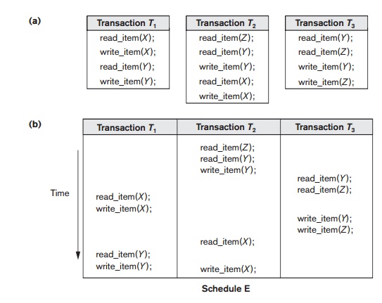
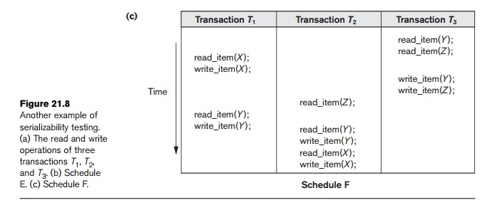
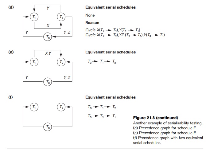
Another example, in which three transactions participate, is shown in Figure 21.8. Figure 21.8(a) shows the read_item and write_item operations in each transaction. Two schedules E and F for these transactions are shown in Figure 21.8(b) and (c),

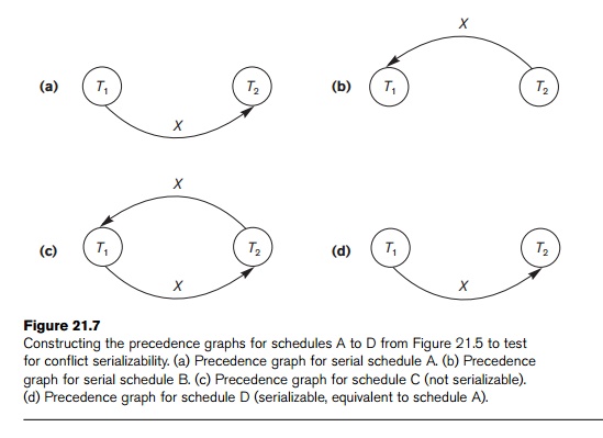
Figure 21.7

Constructing the precedence graphs for schedules A to D from Figure 21.5 to test for conflict serializability. (a) Precedence graph for serial schedule A. (b) Precedence graph for serial schedule B. (c) Precedence graph for schedule C (not serializable). (d) Precedence graph for schedule D (serializable, equivalent to schedule A).

respectively, and the precedence graphs for schedules E and F are shown in parts (d) and (e). Schedule E is not serializable because the corresponding precedence graph has cycles. Schedule F is serializable, and the serial schedule equivalent to F is shown in Figure 21.8(e). Although only one equivalent serial schedule exists for F, in general there may be more than one equivalent serial schedule for a serializable sched-ule. Figure 21.8(f) shows a precedence graph representing a schedule that has two equivalent serial schedules. To find an equivalent serial schedule, start with a node that does not have any incoming edges, and then make sure that the node order for every edge is not violated.

3. How Serializability Is Used for Concurrency Control

As we discussed earlier, saying that a schedule S is (conflict) serializable—that is, S is (conflict) equivalent to a serial schedule—is tantamount to saying that S is correct. Being serializable is distinct from being serial, however. A serial schedule represents inefficient processing because no interleaving of operations from different transac-tions is permitted. This can lead to low CPU utilization while a transaction waits for disk I/O, or for another transaction to terminate, thus slowing down processing considerably. A serializable schedule gives the benefits of concurrent execution without giving up any correctness. In practice, it is quite difficult to test for the seri-alizability of a schedule. The interleaving of operations from concurrent transac-tions—which are usually executed as processes by the operating system—is typically determined by the operating system scheduler, which allocates resources to

all processes. Factors such as system load, time of transaction submission, and priorities of processes contribute to the ordering of operations in a schedule. Hence, it is difficult to determine how the operations of a schedule will be interleaved before-hand to ensure serializability.

If transactions are executed at will and then the resulting schedule is tested for serializability, we must cancel the effect of the schedule if it turns out not to be serializable. This is a serious problem that makes this approach impractical. Hence, the approach taken in most practical systems is to determine methods or protocols that ensure serializability, without having to test the schedules themselves. The approach taken in most commercial DBMSs is to design protocols (sets of rules) that—if fol-lowed by every individual transaction or if enforced by a DBMS concurrency control subsystem—will ensure serializability of all schedules in which the transactions participate.

Another problem appears here: When transactions are submitted continuously to the system, it is difficult to determine when a schedule begins and when it ends. Serializability theory can be adapted to deal with this problem by considering only the committed projection of a schedule S. Recall from Section 21.4.1 that the committed projection C(S) of a schedule S includes only the operations in S that belong to committed transactions. We can theoretically define a schedule S to be serializable if its committed projection C(S) is equivalent to some serial schedule, since only committed transactions are guaranteed by the DBMS.

In Chapter 22, we discuss a number of different concurrency control protocols that guarantee serializability. The most common technique, called two-phase locking, is based on locking data items to prevent concurrent transactions from interfering with one another, and enforcing an additional condition that guarantees serializability. This is used in the majority of commercial DBMSs. Other protocols have been proposed;¹⁴ these include timestamp ordering, where each transaction is assigned a unique timestamp and the protocol ensures that any conflicting opera-tions are executed in the order of the transaction timestamps; multiversion protocols, which are based on maintaining multiple versions of data items; and optimistic (also called certification or validation) protocols, which check for possible serializability violations after the transactions terminate but before they are permitted to commit.

4. View Equivalence and View Serializability

In Section 21.5.1 we defined the concepts of conflict equivalence of schedules and conflict serializability. Another less restrictive definition of equivalence of schedules is called view equivalence. This leads to another definition of serializability called view serializability. Two schedules S and S are said to be view equivalent if the fol-lowing three conditions hold:

        1. The same set of transactions participates in S and S , and S and S include the same operations of those transactions.

       2. For any operation r_i(X) of T_i in S, if the value of X read by the operation has been written by an operation w_j(X) of T_j (or if it is the original value of X before the schedule started), the same condition must hold for the value of X read by operation r_i(X) of T_i in S .

        3. If the operation w_k(Y) of T_k is the last operation to write item Y in S, then w_k(Y) of T_k must also be the last operation to write item Y in S .

The idea behind view equivalence is that, as long as each read operation of a trans-action reads the result of the same write operation in both schedules, the write operations of each transaction must produce the same results. The read operations are hence said to see the same view in both schedules. Condition 3 ensures that the final write operation on each data item is the same in both schedules, so the data-base state should be the same at the end of both schedules. A schedule S is said to be view serializable if it is view equivalent to a serial schedule.

The definitions of conflict serializability and view serializability are similar if a condition known as the constrained write assumption (or no blind writes) holds on all transactions in the schedule. This condition states that any write operation w_i(X) in T_i is preceded by a r_i(X) in T_i and that the value written by w_i(X) in T_i depends only on the value of X read by r_i(X). This assumes that computation of the new value of X is a function f(X) based on the old value of X read from the database. A blind write is a write operation in a transaction T on an item X that is not dependent on the value of X, so it is not preceded by a read of X in the transaction T.

The definition of view serializability is less restrictive than that of conflict serializability under the unconstrained write assumption, where the value written by an operation w_i(X) in T_i can be independent of its old value from the database. This is possible when blind writes are allowed, and it is illustrated by the following schedule S_g of three transactions T₁: r₁(X); w₁(X); T₂: w₂(X); and T₃: w₃(X):

S_g: r₁(X); w₂(X); w₁(X); w₃(X); c₁; c₂; c₃;

In S_g the operations w₂(X) and w₃(X) are blind writes, since T₂ and T₃ do not read the value of X. The schedule S_g is view serializable, since it is view equivalent to the serial schedule T₁, T₂, T₃. However, S_g is not conflict serializable, since it is not conflict equivalent to any serial schedule. It has been shown that any conflict-serializable schedule is also view serializable but not vice versa, as illustrated by the preceding example. There is an algorithm to test whether a schedule S is view serializable or not. However, the problem of testing for view serializability has been shown to be NP-hard, meaning that finding an efficient polynomial time algorithm for this problem is highly unlikely.

5. Other Types of Equivalence of Schedules

Serializability of schedules is sometimes considered to be too restrictive as a condition for ensuring the correctness of concurrent executions. Some applications can produce schedules that are correct by satisfying conditions less stringent than either conflict serializability or view serializability. An example is the type of transactions known as debit-credit transactions—for example, those that apply deposits and withdrawals to a data item whose value is the current balance of a bank account. The semantics of debit-credit operations is that they update the value of a data item X by either subtracting from or adding to the value of the data item. Because addition and subtraction operations are commutative—that is, they can be applied in any order—it is possible to produce correct schedules that are not serializable. For example, consider the following transactions, each of which may be used to transfer an amount of money between two bank accounts:

T₁: r₁(X); X := X − 10; w₁(X); r₁(Y); Y := Y + 10; w₁(Y); T₂: r₂(Y); Y := Y − 20; w₂(Y); r₂(X); X := X + 20; w₂(X);

Consider the following nonserializable schedule S_h for the two transactions: S_h: r₁(X); w₁(X); r₂(Y); w₂(Y); r₁(Y); w₁(Y); r₂(X); w₂(X);

With the additional knowledge, or semantics, that the operations between each r_i(I) and w_i(I) are commutative, we know that the order of executing the sequences consisting of (read, update, write) is not important as long as each (read, update, write) sequence by a particular transaction T_i on a particular item I is not interrupted by conflicting operations. Hence, the schedule S_h is considered to be correct even though it is not serializable. Researchers have been working on extending concurrency control theory to deal with cases where serializability is considered to be too restrictive as a condition for correctness of schedules. Also, in certain domains of applications such as computer aided design (CAD) of complex systems like aircraft, design transactions last over a long time period. In such applications, more relaxed schemes of concurrency control have been proposed to maintain consistency of the database.