Chapter: Operations Research: An Introduction : Deterministic Dynamic Programming
Recursive Nature of Computations in DP(Dynamic Programming)
RECURSIVE NATURE OF COMPUTATIONS IN DP
Computations
in DP are done recursively, so that the optimum solution of one subproblem is
used as an input to the next subproblem. By the time the last subproblem is
solved, the optimum solution for the entire problem is at hand. The manner in
which the recursive computations are carried out depends on how we decompose
the original problem. In particular, the subproblems are normally linked by
common constraints. As we move from one subproblem to the next, the feasibility
of these common constraints must be maintained.
Example
10.1-1 (Shortest-Route Problem)
Suppose
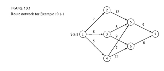
that you want to select the shortest highway route between two cities. The
network in Figure 10.1 provides the possible routes between the starting city
at node 1 and the destination city at node 7. The routes pass through
intermediate cities designated by nodes 2 to 6.
We can
solve this problem by exhaustively enumerating all the routes between nodes 1
and 7 (there are five such routes). However, in a large network, exhaustive
enumeration may be intractable computationally. '
To solve
the problem by DP, we first decompose it into stages as delineated by the
vertical dashed lines in Figure 10.2. Next, we carry out the computations for
each stage separately.
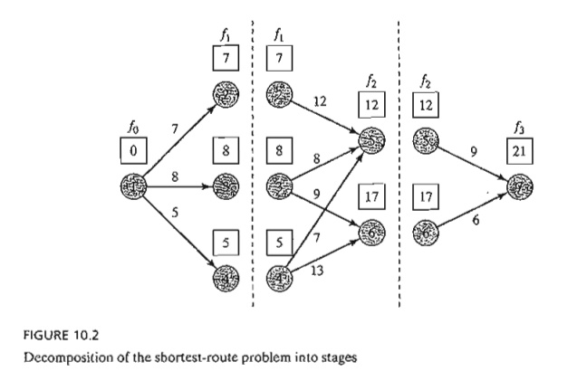
The
general idea for determining the shortest route is to compute the shortest
(cumulative) distances to all the terminal nodes of a stage and then use these
distances as input data to the immediately succeeding stage. Starting from node
1, stage 1 includes three end nodes (2,3, and 4) and its computations are
simple.
Stage 1 Summary.
Shortest
distance from node 1 to node 2 = 7 miles (from
node 1)
Shortest
distance from node 1 to node 3 = 8 miles (from
node 1)
Shortest
distance from node 1 to node 4 = 5 miles (from
node 1)
Next,
stage 2 has two end nodes, 5 and 6. Considering node 5 first, we see from
Figure 10.2 that node 5 can be reached from three nodes, 2,3, and 4, by three
different routes: (2,5), (3,5), and (4, 5). This information, together with the
shortest distances to nodes 2, 3, and 4, determines the shortest (cumulative)
distance to node 5 as
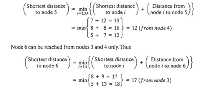
Stage 2 Summary.
Shortest
distance from node 1 to node 5 = 12 miles (from
node 4)
Shortest
distance from node 1 to node 6 = 17 miles (from
node 3)
The last
step is to consider stage 3. The destination node 7 can be reached from either
nodes 5 or 6. Using the summary results from stage 2 and the distances from
nodes 5 and 6 to node 7, we get
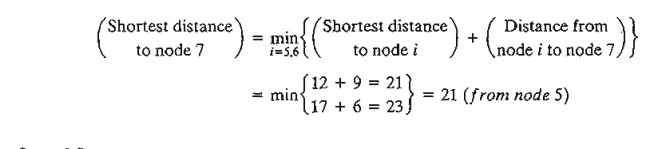
Stage 3 Summary.
Shortest
distance from node 1 to node 7 = 21 miles (from
node 5)
Stage 3
summary shows that the shortest distance between nodes 1 and 7 is 21 miles. To
deter-mine the optimal route, stage 3 summary links node 7 to node 5, stage 2
summary links node 4 to node 5, and stage 1 summary links node 4 to node 1.
Thus, the shortest route is 1 - > 4 -
> 5 - > 7.
The
example reveals the basic properties of computations in DP:
a)
The computations at each stage are a function of
the feasible routes of that stage, and that stage alone.
b)
A current stage is linked to the immediately preceding stage only without
regard to earlier stages. The linkage is in the form of the shortest-distance
summary that represents the out-put of the immediately preceding stage.
Recursive Equation. We now
show how the recursive computations in Example 10.1-1 can be expressed
mathematically. Let fi(xi)
be the shortest distance to node xi
at stage 4 and define d(xi-1,
xi) as the distance from node xi-l to node xi, then fi is computed from fi-1 using the following
recursive equation:

Starting
at i = 1, the recursion sets fo(xo) = 0. The equation shows that the
shortest distances fi(xj)
at stage i must be expressed in terms
of the next node, xi. In
the DP terminology, xi is
referred to as the state of the system at stage i. In effect, the state of
the system at stage i is the information that links the
stages together, so that optimal
decisions for the remaining stages can be made without reexamining how the
decisions for the previous stages are reached. The proper definition of the state allows us to consider each stage
separately and guarantee that the solution is feasible for all the stages.
The
definition of the state leads to the
following unifying framework for DP.
Principle of Optimality
Future decisions for the remaining stages will constitute an optimal
policy regardless of the policy adopted in previous stages.
The
implementation of the principle is evident in the computations in Example
10.1-1. For example, in stage 3, we only use the shortest distances to nodes 5
and 6, and do not concern ourselves with how these nodes are reached from node 1. Although the principle of
optimality is "vague" about the details of how each stage is
optimized, its application greatly facilitates the solution of many complex
problems.
PROBLEM SET 10.lA
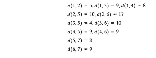
*1. Solve Example 10.1-1, assuming the following routes are used:
2. I am an avid hiker. Last summer, I went with my friend G. Don on a 5-day hike-and-camp trip in the beautiful White Mountains in
New Hampshire. We decided to limit our hiking to an area comprising three
well-known peaks: Mounts Washington, Jefferson, and Adams. Mount Washington has
a 6-mile base-to-peak trail. The corresponding base-ta-peak trails for Mounts
Jefferson and Adams are 4 and 5 miles, respectively. The trails joining the
bases of the three mountains are 3 miles between Mounts Washington and
Jefferson, 2 miles between Mounts Jefferson and Adams, and 5 miles between
Mounts Adams and Washington. We started on the first day at the base of Mount
Washington and returned to the same spot at the end of 5 days. Our goal was to
hike as many miles as we could. We also decided to climb exactly one mountain
each day and to camp at the base of the moun-tain we would be climbing the next
day. Additionally, we decided that the same mountain could not be visited in
any two consecutive days. How did we schedule our hike?
Related Topics