Linear Simple Harmonic Oscillator (LHO)

LINEAR SIMPLE HARMONIC OSCILLATOR (LHO)

Horizontal oscillations of a spring-mass system

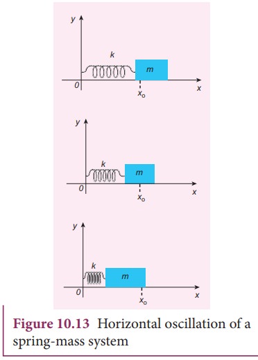
Consider a system containing a block of mass m attached to a massless spring with stiffness constant or force constant or spring constant k placed on a smooth horizontal surface (frictionless surface) as shown in Figure 10.13. Let x₀ be the equilibrium position or mean position of mass m when it is left undisturbed. Suppose the mass is displaced through a small displacement x towards right from its equilibrium position and then released, it will oscillate back and forth about its mean position x₀. 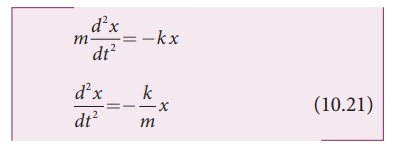Let F be the restoring force (due to stretching of the spring) which is proportional to the amount of displacement of block. For one dimensional motion, mathematically, we have

where negative sign implies that the restoring force will always act opposite to the direction of the displacement. This equation is called Hooke’s law. Notice that, the restoring force is linear with the displacement (i.e., the exponent of force and displacement are unity). This is not always true; in case if we apply a very large stretching force, then the amplitude of oscillations becomes very large (which means, force is proportional to displacement containing higher powers of x) and therefore, the oscillation of the system is not linear and hence, it is called non-linear oscillation. We restrict ourselves only to linear oscillations throughout our discussions, which means Hooke’s law is valid (force and displacement have a linear relationship).

From Newton’s second law, we can write the equation for the particle executing simple harmonic motion

Comparing the equation (10.21) with simple harmonic motion equation (10.10), we get

which means the angular frequency or natural frequency of the oscillator is

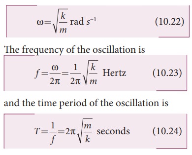
Notice that in simple harmonic motion, the time period of oscillation is independent of amplitude. This is valid only if the amplitude of oscillation is small.

The solution of the differential equation of a SHM may be written as

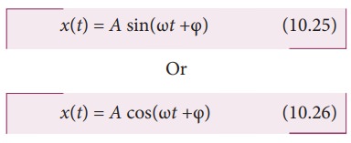
where A, ω and ϕ are constants. General solution for differential equation 10.21 is x(t) = A sin(ωt +φ)+ B cos(ωt +φ) where A and B are contants.

Vertical oscillations of a spring

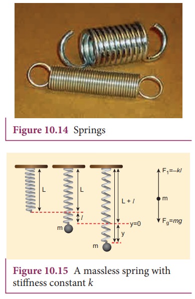
Let us consider a massless spring with stiffness constant or force constant k attached to a ceiling as shown in Figure 10.15. Let the length of the spring before loading mass m be L. If the block of mass m is attached to the other end of spring, then the spring elongates by a length l. Let F₁ be the restoring force due to stretching of spring. Due to mass m, the gravitational force acts vertically downward. 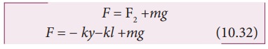We can draw free-body diagram for this system as shown in Figure 10.15. When the system is under equilibrium,

But the spring elongates by small displacement l, therefore,

Substituting equation (10.28) in equation (10.27), we get

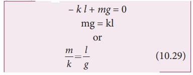
Suppose we apply a very small external force on the mass such that the mass further displaces downward by a displacement y, then it will oscillate up and down. Now, the restoring force due to this stretching of spring (total extension of spring is y + l ) is

Since, the mass moves up and down with acceleration d²y/dt², by drawing the free body, diagram for this case, we get

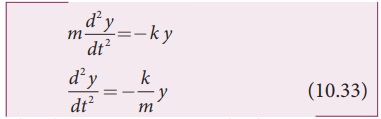
The net force acting on the mass due to this stretching is

The gravitational force opposes the restoring force. Substituting equation (10.29) in equation (10.32), we get

F = −ky − kl + kl = −ky

Applying Newton’s law, we get

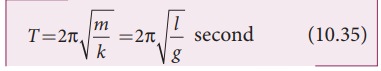
The above equation is in the form of simple harmonic differential equation. Therefore, we get the time period as

The time period can be rewritten using equation (10.29)

The acceleration due to gravity g can be computed from the formula

EXAMPLE 10.8

A spring balance has a scale which ranges from 0 to 25 kg and the length of the scale is 0.25m. It is taken to an unknown planet X where the acceleration due to gravity is 11.5 m s⁻¹. Suppose a body of mass M kg is suspended in this spring and made to oscillate with a period of 0.50 s. Compute the gravitational force acting on the body.

Solution

Let us first calculate the stiffness constant of the spring balance by using equation (10.29),

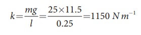
The time period of oscillations is given by T=2π√M/√k, , where M is the mass of the body.

Since, M is unknown, rearranging, we get

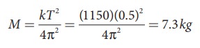
The gravitational force acting on the body is W = Mg = 7.3 × 11.5 = 83.95 N ≈ 84 N

Combinations of springs

Spring constant or force constant, also called as stiffness constant, is a measure of the stiffness of the spring. Larger the value of the spring constant, stiffer is the spring. This implies that we need to apply more force to compress or elongate the spring. Similarly, smaller the value of spring constant, the spring can be stretched (elongated) or compressed with lesser force. Springs can be connected in two ways. Either the springs can be connected end to end, also known as series connection, or alternatively, connected in parallel. In the following subsection, we compute the effective spring constant when

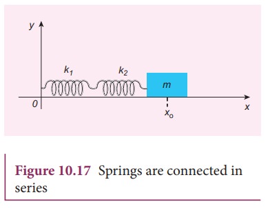
a. Springs are connected in series

b. Springs are connected in parallel

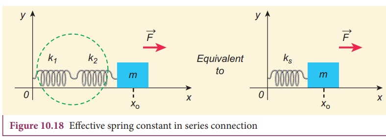
a. Springs connected in series

When two or more springs are connected in series, we can replace (by removing) all the springs in series with an equivalent spring (effective spring) whose net effect is the same as if all the springs are in series connection. Given the value of individual spring constants k₁, k₂, k₃,... (known quantity), we can establish a mathematical relationship to find out an effective (or equivalent) spring constant k_s (unknown quantity). For simplicity, let us consider only two springs whose spring constant are k₁ and k₂ and which can be attached to a mass m as shown in Figure 10.17. The results thus obtained can be generalized for any number of springs in series.

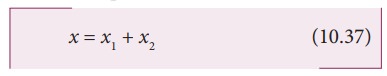
Let F be the applied force towards right as shown in Figure 10.18. Since the spring constants for different spring are different and the connection points between them is not rigidly fixed, the strings can stretch in different lengths. Let x₁ and x₂ be the elongation of springs from their equilibrium position (un-stretched position) due to the applied force F. Then, the net displacement of the mass point is

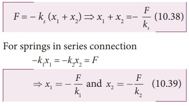
From Hooke’s law, the net force

For springs in series connection

−k1x1 = −k2x2 = F

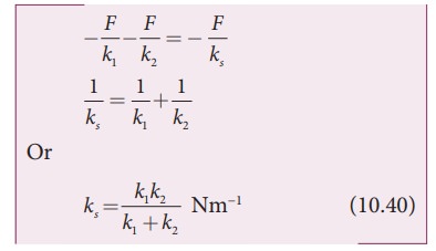
Therefore, substituting equation (10.39) in equation (10.38), the effective spring constant can be calculated as

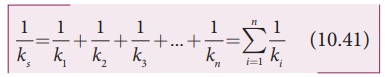
Suppose we have n springs connected in series, the effective spring constant in series is

If all spring constants are identical i.e., k₁ = k₂ =... = k_n = k then

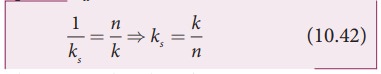
This means that the effective spring constant reduces by the factor n. Hence, for springs in series connection, the effective spring constant is lesser than the individual spring constants.

From equation (10.39), we have,

k₁x₁ = k₂x₂

Then the ratio of compressed distance or elongated distance x₁ and x₂ is

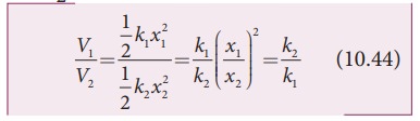
The elastic potential energy stored in first and second springs are V₁=1/2 k₁x₁² and V₂=1/2 k₂x₂² respectively. Then, their ratio is

EXAMPLE 10.9

Consider two springs whose force constants are 1 N m⁻¹ and 2 N m⁻¹ which are connected in series. Calculate the effective spring constant (k_s ) and comment on k_s .

Solution

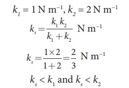
k_s < k₁ and k_s < k

Therefore, the effective spring constant is lesser than both k₁ and k₂.

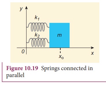
b. Springs connected in parallel

When two or more springs are connected in parallel, we can replace (by removing) all these springs with an equivalent spring (effective spring) whose net effect is same as if all the springs are in parallel connection. Given the values of individual spring constants to be k₁,k₂,k₃, ... (known quantities), we can establish a mathematical relationship to find out an effective (or equivalent) spring constant k_p (unknown quantity). For simplicity, let us consider only two springs of spring constants k₁and k₂ attached to a mass m as shown in Figure 10.19. The results can be generalized to any number of springs in parallel.

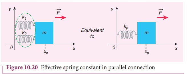
Let the force F be applied towards right as shown in Figure 10.20. In this case, both the springs elongate or compress by the same amount of displacement. Therefore, net force for the displacement of mass m is

where k_p is called effective spring constant. Let the first spring be elongated by a displacement x due to force F₁ and second spring be elongated by the same displacement x due to force F₂, then the net force

Equating equations (10.46) and (10.45), we get

Generalizing, for n springs connected in parallel,

If all spring constants are identical i.e., k₁ = k₂= ... = k_n = k then

This implies that the effective spring constant increases by a factor n. Hence, for the springs in parallel connection, the effective spring constant is greater than individual spring constant.

EXAMPLE 10.10

Consider two springs with force constants 1 N m⁻¹ and 2 N m⁻¹ connected in parallel. Calculate the effective spring constant (k_p ) and comment on k_p.

Solution

k₁ = 1 N m⁻¹, k₂ = 2 N m⁻¹

k_p = k₁ + k₂ N m⁻¹

k_p = 1 + 2 = 3 N m⁻¹

k_p > k₁ and k_p > k₂

Therefore, the effective spring constant is greater than both k₁ and k₂.

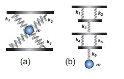
EXAMPLE 10.11

Calculate the equivalent spring constant for the following systems and also compute if all the spring constants are equal:

Solution

a. Since k₁ and k₂ are parallel, k_u = k₁ + k₂ Similarly, k₃ and k₄ are parallel, therefore, k_d = k₃ + k₄

But k_u and k_d are in series,

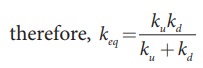
If all the spring constants are equal then, k₁ = k₂ = k₃ = k₄ = k

Which means, k_u = 2k and k_d = 2k

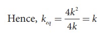
b. Since k₁ and k₂ are parallel, k_A = k₁ + k₂ Similarly, k₄ and k₅ are parallel, therefore, k_B = k₄ + k₅

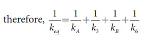
But k_A, k₃, k_B, and k₆ are in series,

If all the spring constants are equal then, k₁ = k₂ = k₃ = k₄ = k₅ = k₆ = k which means, k_A = 2k and k_B = 2k

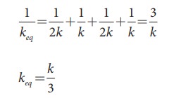
k_eq = k/3

EXAMPLE 10.12

A mass m moves with a speed v on a horizontal smooth surface and collides with a nearly massless spring whose spring constant is k. If the mass stops after collision, compute the maximum compression of the spring.

Solution

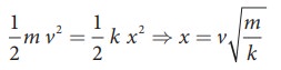
When the mass collides with the spring, from the law of conservation of energy “the loss in kinetic energy of mass is gain in elastic potential energy by spring”.

Let x be the distance of compression of spring, then the law of conservation of energy

Oscillations of a simple pendulum in SHM and laws of simple pendulum

Simple pendulum

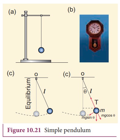
A pendulum is a mechanical system which exhibits periodic motion. It has a bob with mass m suspended by a long string (assumed to be massless and inextensible string) and the other end is fixed on a stand as shown in Figure 10.21 (a). At equilibrium, the pendulum does not oscillate and hangs vertically downward. Such a position is known as mean position or equilibrium position. When a pendulum is displaced through a small displacement from its equilibrium position and released, the bob of the pendulum executes to and fro motion. Let l be the length of the pendulum which is taken as the distance between the point of suspension and the centre of gravity of the bob. Two forces act on the bob of the pendulum at any displaced position, as shown in the Figure 10.21 (d),

(i) The gravitational force acting on the body (  ) which acts vertically downwards.

(ii) The tension in the string  which acts along the string to the point of suspension.

Resolving the gravitational force into its components:

a. Normal component: The component along the string but in opposition to the direction of tension, F_as = mg cosθ.

b. Tangential component: The component perpendicular to the string i.e., along tangential direction of arc of swing, F_ps = mg sinθ.

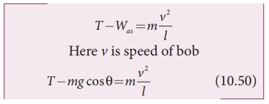
Therefore, The normal component of the force is, along the string,

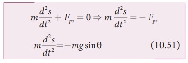
From the Figure 10.21, we can observe that the tangential component W_ps of the gravitational force always points towards the equilibrium position i.e., the direction in which it always points opposite to the direction of displacement of the bob from the mean position. Hence, in this case, the tangential force is nothing but the restoring force. Applying Newton’s second law along tangential direction, we have

where, s is the position of bob which is measured along the arc. Expressing arc length in terms of angular displacement i.e.,

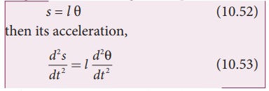
Substituting equation (10.53) in equation (10.51), we get

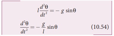
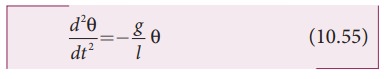
Because of the presence of sin θ in the above differential equation, it is a non-linear differential equation (Here, homogeneous second order). Assume “the small oscillation approximation”, sin θ ≈ θ, the above differential equation becomes linear differential equation.

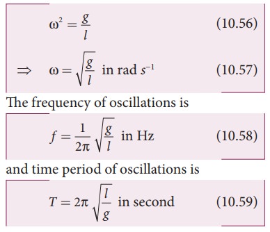
This is the well known oscillatory differential equation. Therefore, the angular frequency of this oscillator (natural frequency of this system) is

Laws of simple pendulum

The time period of a simple pendulum

a. Depends on the following laws

(i) Law of length

For a given value of acceleration due to gravity, the time period of a simple pendulum is directly proportional to the square root of length of the pendulum.

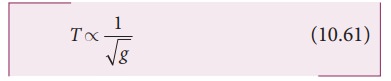
(ii) Law of acceleration

For a fixed length, the time period of a simple pendulum is inversely proportional to square root of acceleration due to gravity.

b. Independent of the following factors

(i) Mass of the bob

The time period of oscillation is independent of mass of the simple pendulum. This is similar to free fall. Therefore, in a pendulum of fixed length, it does not matter whether an elephant swings or an ant swings. Both of them will swing with the same time period.

(ii) Amplitude of the oscillations

For a pendulum with small angle approximation (angular displacement is very small), the time period is independent of amplitude of the oscillation.

EXAMPLE 10.13

In simple pendulum experiment, we have used small angle approximation . Discuss the small angle approximation.

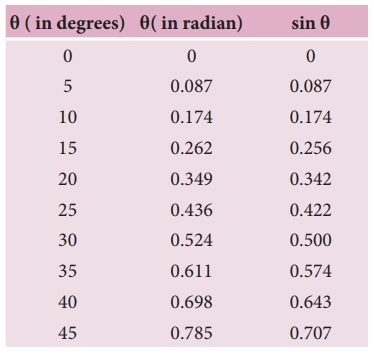
For θ in radian, sin θ ≈ θ for very small angles

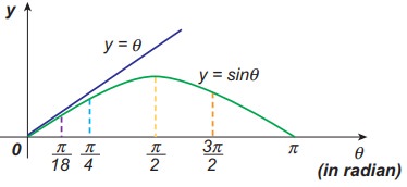
This means that “for θ as large as 10 degrees, sin θ is nearly the same as θ when θ  is expressed in radians”. As θ increases in value sinθ gradually becomes different from θ

Pendulum length due to effect of temperature

Suppose the suspended wire is affected due to change in temperature. The rise in temperature affects length by

l = l_o (1 + α ∆t)

where l_o is the original length of the wire and l is final length of the wire when the temperature is raised. Let ∆t is the change in temperature and α is the co-efficient of linear expansion.

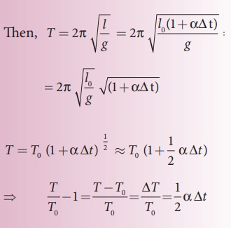
where ∆T is the change in time period due to the effect of temperature and T₀ is the time period of the simple pendulum with original length l₀.

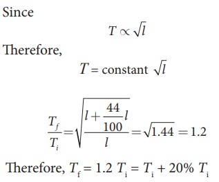
EXAMPLE 10.14

If the length of the simple pendulum is increased by 44% from its original length, calculate the percentage increase in time period of the pendulum.

Solution

Oscillation of liquid in a U-tube:

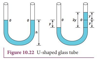
Consider a U-shaped glass tube which consists of two open arms with uniform cross-sectional area A. Let us pour a non-viscous uniform incompressible liquid of density ρ in the U-shaped tube to a height h as shown in the Figure 10.22. If the liquid and tube are not disturbed then the liquid surface will be in equilibrium position O. It means the pressure as measured at any point on the liquid is the same and also at the surface on the arm (edge of the tube on either side), which balances with the atmospheric pressure. Due to this the level of liquid in each arm will be the same. By blowing air one can provide sufficient force in one arm, and the liquid gets disturbed from equilibrium position O, which means, the pressure at blown arm is higher than the other arm. This creates difference in pressure which will cause the liquid to oscillate for a very short duration of time about the mean or equilibrium position and finally comes to rest.

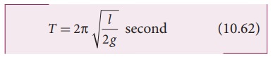
Time period of the oscillation is