Visual Realism

Visual Realism

Introduction

Visual Realism is a method for interpreting picture data fed into a computer and for creating pictures from difficult multidimensional data sets. Visualization can be classified as :

·       Visualization in geometric modeling

·       Visualization in scientific computing.

Visualization in geometric modeling is helpful in finding connection in the design applications. By shading the parts with various shadows, colors and transparency, the designer can recognize undesired unknown interferences. In the design of complex surfaces shading with different texture characteristics can use to find any undesired quick modifications in surface changes.

Visualization in computing is viewed as a technique of geometric modeling. It changes the data in numerical form into picture display, allowing users to view their simulations and computations. Visualization offers a process of seeing the hidden. Visualization in scientific computing is of great interest to engineers during the design process.

Existing visualization methods are:

·       Parallel projections

·       Perspective projection.

·       Hidden line removal

·       Hidden surface removal

·       Hidden solid removal

·       Shaded models

Hidden line and surface removal methods remove the uncertainty of the displays of 3D models and is accepted the first step towards visual realism. Shaded images can only be created for surface and solid models. In multiple step shading process, the first step is removing the hidden surfaces / solids and second step is shades the visible area only. Shaded images provide the maximum level of visualization.

The processes of hidden removal need huge amounts of computing times and also upper end hardware services. The creation and maintenance of such a models are become complex. Hence, creating real time images needs higher end computers with the shading algorithms embedded into the hardware.

Hidden line removal

Hidden line removal (HLR) is the method of computing which edges are not hidden by the faces of parts for a specified view and the display of parts in the projection of a model into a 2D plane. Hidden line removal is utilized by a CAD to display the visual lines. It is considered that information openly exists to define a 2D wireframe model as well as the 3D topological information. Typically, the best algorithm is required for viewing this information from an available part representation.

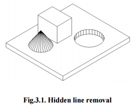
Fig.3.1. Hidden line removal

3D parts are simply manufactured and frequently happen in a CAD design of such a part. In addition, the degrees of freedom are adequate to show the majority of models and are not overwhelming in the number of constraints to be forced. Also, almost all the surface-surface intersections and shadow computations can be calculated analytically which results in significant savings in the number of computations over numerical methods.

 1. Priority algorithm

Priority algorithm is basis on organization all the polygons in the view according to the biggest Z-coordinate value of each. If a face intersects more than one face, other visibility tests besides the Z-depth required to solve any issue. This step comprises purposes of wrapper.

Imagines that objects are modeled with lines and lines are generated where surfaces join. If only the visible surfaces are created then the invisible lines are automatically removed.

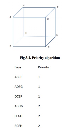
Fig.3.2. Priority algorithm

Face   Priority

ABCE   1

ADFG 1

DCEF  1

ABHG 2

EFGH  2

BCEH  2

ABCD, ADFG, DCEF are given higher priority-1. Hence, all lines in this faces are visible, that is, AB, BC, CD, DA, AD, DF, FG, AG, DC, CE, EF and DF are visible.

AGHB, EFGH, BCEH are given lower priority-2. Hence, all lines in this faces other than priority-1 are invisible, that is BH, EH and GH. These lines must be eliminated.

Hidden surface removal

The hidden surface removal is the procedure used to find which surfaces are not visible from a certain view. A hidden surface removal algorithm is a solution to the visibility issue, which was one of the first key issues in the field of three dimensional graphics. The procedure of hidden surface identification is called as hiding, and such an algorithm is called a ‘hider’.Hidden surface identification is essential to render a 3D image properly, so that one cannot see through walls in virtual reality.

Hidden surface identification is a method by which surfaces which should not be visible to the user are prohibited from being rendered. In spite of benefits in hardware potential there is still a requirement for difficult rendering algorithms. The accountability of a rendering engine is to permit for bigger world spaces and as the world’ssize approaches infinity the rendering engine should not slow down but maintain at constant speed.

There are many methods for hidden surface identification. They are basically a work out in sorting, and generally vary in the order in which the sort is executed and how the problem is subdivided. Sorting more values of graphics primitives is generally done by divide.

1. Z - buffer algorithm

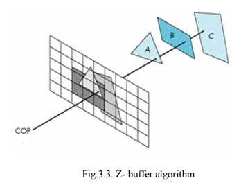
Fig.3.3. Z- buffer algorithm

In Z-buffering, the depth of ‘Z’value is verified against available depth value. If the present pixel is behind the pixel in the Z-buffer, the pixel is eliminated, or else it is shaded and its depth value changes the one in the Z-buffer. Z-buffering helps dynamic visuals easily, and is presently introduced effectively in graphics hardware.

·        Depth buffering is one of the easiest hidden surface algorithms

·        It keeps follow of the space to nearest object at every pixel position.

·       Initialized to most negative z value.

·        when image being drawn, if its z coordinate at a position is higher than z buffer value, it is drawn, and new z coordinate value is stored; or else, it is not drawn

·        If a line in three dimensional is being drawn, then the middle z values are interpolated: linear interpolation for polygons, and can calculate z for more difficult surfaces.

Algorithm: loop on y;

loop on x;

zbuf[x,y] = infinity;

loop on objects

{

loop on y within y range of this object

{

loop on x within x range of this scan line of this object

{

if z(x,y) < zbuf[x,y] compute z of this object at this pixel & test zbuf[x,y] = z(x,y) update z-buffer

image[x,y] = shade(x,y) update image (typically RGB)

}

}

}

Basic operations:

1.    compute y range of an object

2.    compute x range of a given scan line of an object

3.    Calculate intersection point of a object with ray through pixel position (x,y).

2.Painter’salgorithm

The painter's algorithm is called as a priority fill, is one of the easiest results to the visibility issue in three dimensional graphics. When projecting a 3D view onto a 2D screen, it is essential at various points to be finalized which polygons are visible, and which polygons are hidden.

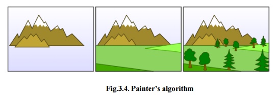
Fig.3.4. Painter’salgorithm

The ‘painter's algorithm’shows to the method employed by most of the painters of painting remote parts of a scene before parts which are close thereby hiding some areas of distant parts. The painter's algorithm arranges all the polygons in a view by their depth and then paints them in this order, extreme to closest. It will paint over the existing parts that are usually not visible hence solving the visibility issue at the cost of having painted invisible areas of distant objects. The ordering used by the algorithm is referred a 'depth order', and does not have to respect the distances to the parts of the scene: the important characteristics of this ordering is, somewhat, that if one object has ambiguous part of another then the first object is painted after the object that it is ambiguous. Thus, a suitable ordering can be explained as a topological ordering of a directed acyclic graph showing between objects.

Algorithm:

sort objects by depth, splitting if necessary to handle intersections; loop on objects (drawing from back to front)

{

loop on y within y range of this object

{

loop on x within x range of this scan line of this object

{

image[x,y] = shade(x,y);

}

}

}

Basic operations:

1.     compute ‘y’range of an object

2.     compute ‘x’range of a given scan line of an object

3.     compute intersection point of  a given object with ray via pixel point (x,y).

4.     evaluate depth of two objects, determine if A is in front of B, or B is in front of A, if they don’t overlap in xy, or if they intersect

5.     divide one object by another object

Advantage of painter's algorithm is the inner loops are quite easy and limitation is sorting

operation.

3. Warnock algorithm

The Warnock algorithm is a hidden surface algorithm developed by John Warnock that is classically used in the area of graphics. It explains the issues of rendering a difficult image by recursive subdivision of a view until regions are attained that is trivial to evaluate. Similarly, if the view is simple to compute effectively then it is rendered; else it is split into tiny parts which are likewise evaluated for simplicity. This is a algorithm with run-time of O(np), where p is the number of pixels in the viewport and n is the number of polygons.

The inputs for Warnock algorithm are detail of polygons and a viewport. The good case is that if the detail of polygons is very simple then creates the polygons in the viewport. The continuous step is to divide the viewport into four equally sized quadrants and to recursively identify the algorithm for each quadrant, with a polygon list changed such that it contains polygons that are detectable in that quadrant.

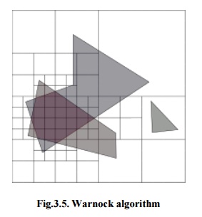
Fig.3.5. Warnock algorithm

1.  Initialize the region.

2.  Generate list of polygons by sorting them with their z values.

3.  Remove polygons which are outside the area.

4.  Identify relationship of each polygon.

5.  Execute visibility decision analysis:

a)Fill area with background color if all polygons are disjoint,

b)Fill entire area with background color and fill part of polygon contained in area with color of polygon if there is only one contained polygon,

c) If there is a single surrounding polygon but not contained then fill area with color of surrounding polygon.

d)Set pixel to the color of polygon which is closer to view if region of the pixel (x,y) and if neither of (a) to (d) applies calculate z- coordinate at pixel (x,y) of polygons.

6.  If none of above is correct then subdivide the area and Go to Step 2.

Hidden Solid Removal

The hidden solid removal issue involves the view of solid models with hidden line or surface eliminated. Available hidden line algorithm and hidden surface algorithms are useable to hidden solid elimination of B-rep models.

The following techniques to display CSG models:

1.    Transfer the CSG model into a boundary model.

2.    Use a spatial subdivision strategy.

3.    Based on ray sorting.

 1.Ray-Tracing algorithm

A ray tracing is a method for creating an image by tracing the path of light via pixels in an image plane and reproducing the effects of its meets with virtual objects. The procedure is capable of creating a high degree of visual realism, generally higher than that of usual scan line techniques, but at a better computational. This creates ray tracing excellent suited for uses where the image can be rendered gradually ahead of time, similar to still images and film and TV visual effects, and more badly suited for real time environment like video games where speed is very important. Ray tracing is simulating a wide range of optical effects, such as scattering, reflection and refraction.

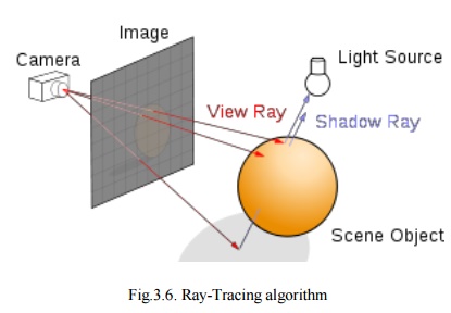
Fig.3.6. Ray-Tracing algorithm

Ray-Tracing algorithm

For every pixel in image

{

Generate ray from eye point passing via this pixel Initialize Nearest ‘T’to ‘INFINITY’

Initialize Nearest Object to NULL

For each object in scene

{

If ray intersects this image

{

If t of intersection is less than Nearest T

{

Set Nearest T to t of the intersection

Set Nearest image to this object

}

}

}

If Nearest image is NULL

{

Paint this pixel with background color

}

Else

{

Shoot a ray to every light source to check if in shadow

If surface is reflective, generate reflection ray

If transparent, generate refraction ray

Apply Nearest Object and Nearest T to execute shading function

Paint this pixel with color result of shading function

}

}

Optical ray tracing explains a technique for creating visual images constructed in three dimensional graphics environments, with higher photorealism than either ray casting rendering practices. It executes by tracing a path from an imaginary eye via every pixel in a virtual display, and computing the color of the object visible via it.

Displays in ray tracing are explained mathematically by a programmer. Displays may also incorporate data from 3D models and images captured like a digital photography.

In general, every ray must be tested for intersection with a few subsets of all the objects in the view. Once the nearest object has been selected, the algorithm will calculate the receiving light at the point of intersection, study the material properties of the object, and join this information to compute the finishing color of the pixel. One of the major limitations of algorithm, the reflective or translucent materials may need additional rays to be re-cast into the scene.

Advantages of Ray tracing:

1.     A realistic simulation of lighting over other rendering.

2.     An effect such as reflections and shadows is easy and effective.

3.     Simple to implement yet yielding impressive visual results.

Limitation of ray tracing:

Scan line algorithms use data consistency to divide computations between pixels, while ray tracing normally begins the process a new, treating every eye ray separately.

Shading

Shading defines to describe depth perception in three dimensioning models by different levels of darkness. Shading is applied in drawing for describes levels of darkness on paper by adding media heavy densely shade for darker regions, and less densely for lighter regions.

There are different techniques of shading with cross hatching where perpendicular lines of changing closeness are drawn in a grid pattern to shade an object. The closer the lines are combining, the darker the area appears. Similarly, the farther apart the lines are, the lighter the area shows.

Fig.3.7. Shading

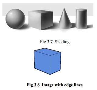
Fig.3.8. Image with edge lines

The image shown in figure 3.8 has the faces of the box rendered, but all in the similar color. Edge lines have been rendered here as well which creates the image easier to view.

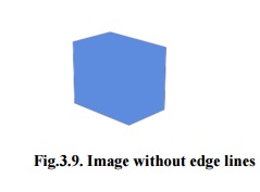
Fig.3.9. Image without edge lines

The image shown in figure 3.9 is the same model rendered without edge lines. It is complicated to advise where one face of the box ends and the next starts.

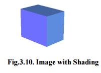
Fig.3.10. Image with Shading

The image shown in figure 3.10 has shading enabled which makes the image extra realistic and makes it easier to view which face is which.

Shading techniques:

In computer graphics, shading submits to the procedure of changing the color of an object in the 3D view, a photorealistic effect to be based on its angle to lights and its distance from lights. Shading is performed through the rendering procedure by a program called a ‘Shader’. Flat shading and Smooth shading are the two major techniques using in Computer graphics.