Uncertainty - Artificial Intelligence

UNCERTAINTY

1. UNCERTAINTY

To act rationally under uncertainty we must be able to evaluate how likely certain things are. With FOL a fact F is only useful if it is known to be true or false. But we need to be able to evaluate how likely it is that F is true. By weighing likelihoods of events (probabilities) we can develop mechanisms for acting rationally under uncertainty.

Dental Diagnosis example.

In FOL we might formulate

P. symptom(P,toothache)→  disease(p,cavity)              disease(p,gumDisease)  

disease(p,foodStuck)                        

When do we stop?

Cannot list all possible causes.

We also want to rank the possibilities. We don’t want to start drilling for a cavity before checking for more likely causes first.

Axioms Of Probability

Given a set U (universe), a probability function is a function defined over the subsets of U that maps each subset to the real numbers and that satisfies the Axioms of Probability

1.Pr(U)  = 1

2.Pr(A)  [0,1]

3.Pr(A   ∈B) = Pr(A) + Pr(B) –Pr(A ∩B)

∪

Note if A ∩B = {} then Pr(A ∪B) = Pr(A) + Pr(B)

2. REVIEW OF PROBABILTY

·                    Natural  way  to  represent  uncertainty

·        People  have  intuitive  notions  about  probabilities

·                    Many  of  these  are  wrong  or  inconsistent

·        Most  people don’t get what probabilities mean

·                    Understanding  Probabilities

·        Initially, probabilities are “relative frequencies”

·        This  works  well  for  dice  and  coin  flips

·                    For  more  complicated  events,  this  is  problematic

·        What  is  the  probability  that  Obama  will  be  reelected?

·                    This  event  only  happens  once

·                    We can’t count frequencies

·                    still  seems  like  a  meaningful  question

·                    In  general,  all  events  are  unique

Probabilities and Beliefs

• Suppose I have flipped a coin and hidden the outcome

• What is P(Heads)?

• Note that this is a statement about a belief, not a statement about the world

• The world is in exactly one state (at the macro level) and it is in that state with probability 1.

• Assigning truth values to probability statements is very tricky business

• Must reference speakers state of knowledge

Frequentism and Subjectivism

• Frequentists hold that probabilities must come from relative frequencies

• This is a purist viewpoint

• This is corrupted by the fact that relative frequencies are often unobtainable

• Often requires complicated and convoluted

• assumptions to come up with probabilities

• Subjectivists: probabilities are degrees of belief

o Taints purity of probabilities

o Ofen more practical

Types are:

1 Unconditional or prior probabilities

2 Conditional or posterior probabilities

3. PROBABILISTIC REASONING

·                    Representing Knowledge in an Uncertain Domain

·                    Belief network used to encode the meaningful dependence between variables. o Nodes represent random variables

o  Arcs represent direct influence

o Nodes have conditional probability table that gives that var's probability given the different states of its parents

o  Is a Directed Acyclic Graph (or DAG)

The Semantics of Belief Networks

·                    To construct net, think of as representing the joint probability distribution.

·                    To infer from net, think of as representing conditional independence statements.

·                    Calculate a member of the joint probability by multiplying individual conditional probabilities:

o  P(X1=x1, . . . Xn=xn) =

o  = P(X1=x1|parents(X1)) * . . . * P(Xn=xn|parents(Xn))

·                    Note: Only have to be given the immediate parents of Xi, not all other nodes:

o  P(Xi|X(i-1),...X1) = P(Xi|parents(Xi))

·                    To incrementally construct a network:

1.                             Decide on the variables

2.                             Decide on an ordering of them

3.                             Do until no variables are left:

a.                                                     Pick a variable and make a node for it

b.                                                     Set its parents to the minimal set of pre-existing nodes

c.                                                      Define its conditional probability

·                    Often, the resulting conditional probability tables are much smaller than the exponential size of the full joint

·                    If don't order nodes by "root causes" first, get larger conditional probability tables

·                    Different tables may encode the same probabilities.

·                    Some canonical distributions that appear in conditional probability tables:

o deterministic logical relationship (e.g. AND, OR) o deterministic numeric relationship (e.g. MIN)

o parameteric relationship (e.g. weighted sum in neural net) o noisy logical relationship (e.g. noisy-OR, noisy-MAX)

Direction-dependent separation or D-separation:

·                    If all undirected paths between 2 nodes are d-separated given evidence node(s) E, then the 2 nodes are independent given E.

·                    Evidence node(s) E d-separate X and Y if for every path between them E contains a node Z that:

o has an arrow in on the path leading from X and an arrow out on the path leading to Y (or vice versa)

o  has arrows out leading to both X and Y

o  does NOT have arrows in from both X and Y (nor Z's children too)

Inference in Belief Networks

·                    Want to compute posterior probabilities of query variables given evidence variables.

·                    Types of inference for belief networks:

o Diagnostic inference: symptoms to causes o Causal inference: causes to symptoms

o                 Intercausal inference:

o                 Mixed inference: mixes those above

Inference in Multiply Connected Belief Networks

·                    Multiply connected graphs have 2 nodes connected by more than one path

·                    Techniques for handling:

o                 Clustering: Group some of the intermediate nodes into one meganode. Pro: Perhaps best way to get exact evaluation.

Con: Conditional probability tables may exponentially increase in size.

o                 Cutset conditioning: Obtain simplier polytrees by instantiating variables as constants.

Con: May obtain exponential number of simplier polytrees.

Pro: It may be safe to ignore trees with lo probability (bounded cutset conditioning).

Stochastic simulation: run thru the net with randomly choosen values for each node (weighed by prior probabilities).

4. BAYESIAN NETWORK

Bayes’ nets:

A technique for describing complex joint distributions (models) using simple, local distributions

(conditional probabilities)

More properly called graphical models

Local interactions chain together to give global indirect interactions

A Bayesian network is a graphical structure that allows us to represent and reason about an uncertain domain. The nodes in a Bayesian network represent a set of random variables,

X=X1;::Xi;:::Xn, from the domain. A set of directed arcs(or links) connects pairs of nodes, Xi!Xj, representing the direct dependencies between variables.

Assuming discrete variables, the strength of the relationship between variables is quantified by conditional probability distributions associated with each node. The only constraint on the arcs allowed in a BN is that there must not be any directed cycles: you cannot return to a node simply by following directed arcs.

Such networks are called directed acyclic graphs, or simply dags. There are a number of steps that a knowledge engineer must undertake when building a Bayesian network. At this stage we will present these steps as a sequence; however it is important to note that in the real-world the process is not so simple.

Nodes and values

First, the knowledge engineer must identify the variables of interest. This involves answering the question: what are the nodes to represent and what values can they take, or what state can they be in? For now we will consider only nodes that take discrete values. The values should be both mutually exclusive and exhaustive , which means that the variable must take on exactly one of these values at a time. Common types of discrete nodes include:

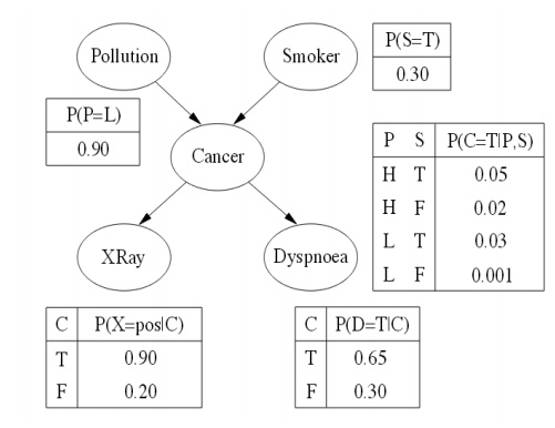
Boolean nodes, which represent propositions, taking the binary values true (T) and false (F). In a medical diagnosis domain, the node Cancer would represent the proposition that a patient has cancer.

Ordered values. For example, a node Pollution might represent a patient’s pol-lution exposure and take the values low, medium, high

Integral values. For example, a node called Age might represent a patient’s age and have possible values from 1 to 120.

Even at this early stage, modeling choices are being made. For example, an alternative to representing a patient’s exact age might be to clump patients into different age groups, such as baby, child, adolescent, young, middleaged, old. The trick is to choose values that represent the domain efficiently.

1 Representation of joint probability distribution

2           Conditional independence relation in Bayesian network

5. INFERENCE IN BAYESIAN NETWORK

1                   Tell

2                   Ask

3                   Kinds of inferences

4                   Use of Bayesian network

·                    In general, the problem of Bayes Net inference is NP-hard (exponential in the size of the graph).

·                    For singly-connected networks or polytrees in which there are no undirected loops, there are linear time algorithms based on belief propagation.

·                    Each node sends local evidence messages to their children and parents.

·                    Each node updates belief in each of its possible values based on incoming messages from it neighbors and propagates evidence on to its neighbors.

·                    There are approximations to inference for general networks based on loopy belief propagation that iteratively refines probabilities that converge to accurate limit.

TEMPORAL MODELS

1                   Monitoring or filtering

2                   Prediction

Bayes' Theorem

Many of the methods used for dealing with uncertainty in expert systems are based on Bayes' Theorem.

Notation:

P(A)  Probability of event A

P(A B) Probability of events A and B occurring together P(A | B) Conditional probability of event A

given that event B has occurred .nr/

If A and B are independent, then P(A | B) = P(A). .co

Expert systems usually deal with events that are not independent, e.g. a disease and its symptoms are not independent.

Theorem

P (A B) = P(A | B)* P(B) = P(B | A) * P(A) therefore P(A | B) = P(B | A) * P(A) / P(B)

Uses of Bayes' Theorem

In doing an expert task, such as medical diagnosis, the goal is to determine identifications (diseases) given observations (symptoms). Bayes' Theorem provides such a relationship.

P(A | B) = P(B | A) * P(A) / P(B)

Suppose: A=Patient has measles,     B =has a rash

Then:P(measles/rash)=P(rash/measles) * P(measles) / P(rash)

The desired diagnostic relationship on the left can be calculated based on the known statistical quantities on the right.

Joint Probability Distribution

Given a set of random variables X1 ... Xn, an atomic event is an assignment of a particular value to each Xi. The joint probability distribution is a table that assigns a probability to each atomic event. Any question of conditional probability can be answered from the joint.

Toothache ¬ Toothache

Cavity  0.04         0.06

¬ Cavity 0.01       0.89

Problems:

The size of the table is combinatoric: the product of the number of possibilities for each random variable. The time to answer a question from the table will also be combinatoric. Lack of evidence: we may not have statistics for some table entries, even though those entries are not impossible.

Chain Rule

We can compute probabilities using a chain rule as follows: P(A &and B &and C) = P(A | B &and C) * P(B | C) * P(C)

If some conditions C1 &and ... &and Cn are independent of other conditions U, we will have:

P(A | C1 &and ... &and Cn &and U) = P(A | C1 &and ... &and Cn)

This allows a conditional probability to be computed more easily from smaller tables using the chain rule.

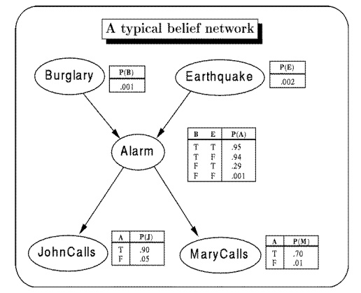
Bayesian Networks

Bayesian networks, also called belief networks or Bayesian belief networks, express relationships among variables by directed acyclic graphs with probability tables stored at the nodes.[Example from Russell & Norvig.]

1                   A burglary can set the alarm off

2                   An earthquake can set the alarm off

3                   The alarm can cause Mary to call

4                   The alarm can cause John to call

Computing with Bayesian Networks

If a Bayesian network is well structured as a poly-tree (at most one path between any two nodes), then probabilities can be computed relatively efficiently. One kind of algorithm, due to Judea Pearl, uses a message-passing style in which nodes of the network compute probabilities and send them to nodes they are connected to. Several software packages exist for computing with belief networks.

A Hidden Markov Model (HMM) tagger chooses the tag for each word that maximizes: [Jurafsky, op. cit.] P(word | tag) * P(tag | previous n tags)

For        a    bigram tagger, this         is       approximated  as:

ti = argmaxj P( wi | tj ) P( tj | ti - 1 )

In practice, trigram taggers are most often used, and a search is made for the best set of tags for the whole sentence; accuracy is about 96%.

6. HIDDEN MARKOV MODELS

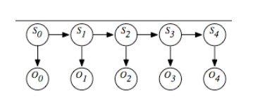
A hidden Markov model (HMM) is an augmentation of the Markov chain to include observations. Just like the state transition of the Markov chain, an HMM also includes observations of the state. These observations can be partial in that different states can map to the same observation and noisy in that the same state can stochastically map to different observations at different times.

The assumptions behind an HMM are that the state at time t+1 only depends on the state at time t, as in the Markov chain. The observation at time t only depends on the state at time t. The observations are modeled using the variable for each time t whose domain is the set of possible observations. The belief network representation of an HMM is depicted in Figure. Although the belief network is shown for four stages, it can proceed indefinitely.

A stationary HMM includes the following probability distributions:

P(S0) specifies initial conditions.

P(St+1|St) specifies the dynamics.

P(Ot|St) specifies the sensor model.

There are a number of tasks that are common for HMMs.

The problem of filtering or belief-state monitoring is to determine the current state based on the current and previous observations, namely to determine P(Si|O0,...,Oi).

Note that all state and observation variables after Si are irrelevant because they are not observed and can be ignored when this conditional distribution is computed.

The problem of smoothing is to determine a state based on past and future observations. Suppose an agent has observed up to time k and wants to determine the state at time i for i<k; the smoothing problem is to determine

P(Si|O0,...,Ok).

All of the variables Si and Vi for i>k can be ignored.