Two n-Body Solvers

TWO n-BODY SOLVERS

In an n-body problem, we need to find the positions and velocities of a collection of interacting particles over a period of time. For example, an astrophysicist might want to know the positions and velocities of a collection of stars, while a chemist might want to know the positions and velocities of a collection of molecules or atoms. An n-body solver is a program that finds the solution to an n-body problem by simulating the behavior of the particles. The input to the problem is the mass, position, and velocity of each particle at the start of the simulation, and the output is typically the position and velocity of each particle at a sequence of user-specified times, or simply the position and velocity of each particle at the end of a user-specified time period.

Let’s first develop a serial n-body solver. Then we’ll try to parallelize it for both shared- and distributed-memory systems.

1. The problem

For the sake of explicitness, let’s write an n-body solver that simulates the motions of planets or stars. We’ll use Newton’s second law of motion and his law of universal gravitation to determine the positions and velocities. Thus, if particle q has position s_q(t) at time t, and particle k has position s_k(t), then the force on particle q exerted by

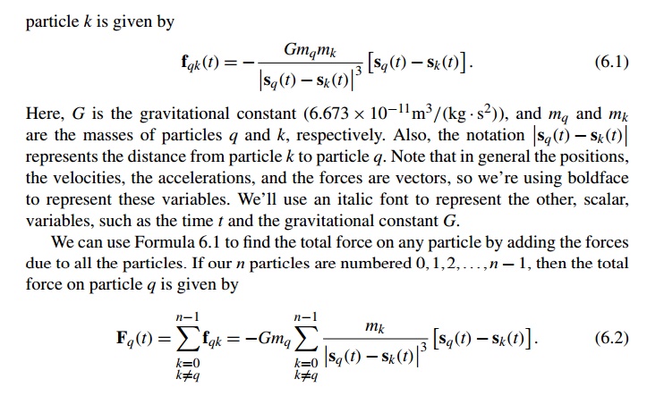
or, more often, simply the positions and velocities at the final time T∆t. Here, ∆t and T are specified by the user, so the input to the program will be n, the number of parti-cles, ∆t, T, and, for each particle, its mass, its initial position, and its initial velocity. In a fully general solver, the positions and velocities would be three-dimensional vec-tors, but in order to keep things simple, we’ll assume that the particles will move in a plane, and we’ll use two-dimensional vectors instead.

The output of the program will be the positions and velocities of the n particles at the timesteps 0, ∆t, 2∆, ...., or just the positions and velocities at T∆t. To get the output at only the final time, we can add an input option in which the user specifies whether she only wants the final positions and velocities.

2. Two serial programs

In outline, a serial n-body solver can be based on the following pseudocode:

            Get input data;

            for each timestep {

            if (timestep output) Print positions and velocities of

particles;

            for each particle q

               Compute total force on q;

            for each particle q

            Compute position and velocity of q;

            }

            Print positions and velocities of particles;

We can use our formula for the total force on a particle (Formula 6.2) to refine our pseudocode for the computation of the forces in Lines 4–5:

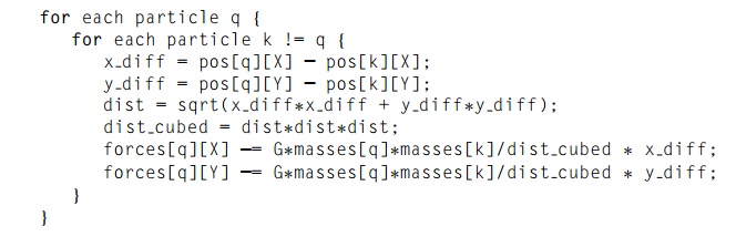
Here, we’re assuming that the forces and the positions of the particles are stored as two-dimensional arrays, forces and pos, respectively. We’re also assuming we’ve defined constants X = 0 and Y = 1. So the x-component of the force on particle q is forces[q][X] and the y-component is forces[q][Y]. Similarly, the compo-nents of the position are pos[q][X] and pos[q][Y]. (We’ll take a closer look at data structures shortly.)

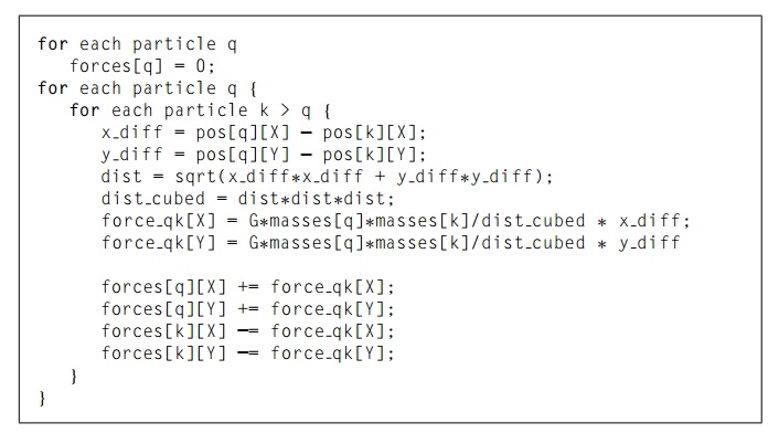
We can use Newton’s third law of motion, that is, for every action there is an equal and opposite reaction, to halve the total number of calculations required for the forces. If the force on particle q due to particle k is f_qk, then the force on k due to q is -f_qk. Using this simplification we can modify our code to compute forces, as shown in Program 6.1. To better understand this pseudocode, imagine the individual forces as a two-dimensional array:

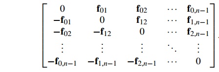
(Why are the diagonal entries 0?) Our original solver simply adds all of the entries in row q to get forces[q]. In our modified solver, when q = 0, the body of the loopp

Program 6.1: A reduced algorithm for computing n-body forces

for each particle q will add the entries in row 0 into forces[0]. It will also add the kth entry in column 0 into forces[k] for k = 1, 2,……., n-1. In general, the qth iteration will add the entries to the right of the diagonal (that is, to the right of the 0) in row q into forces[q], and the entries below the diagonal in column q will be added into their respective forces, that is, the kth entry will be added in to forces[k].

Note that in using this modified solver, it’s necessary to initialize the forces array in a separate loop, since the qth iteration of the loop that calculates the forces will, in general, add the values it computes into forces[k] for k = q + 1, q + 2, …, n-1, not just forces[q].

In order to distinguish between the two algorithms, we’ll call the n-body solver with the original force calculation, the basic algorithm, and the solver with the number of calculations reduced, the reduced algorithm.

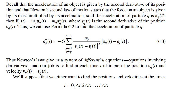
The position and the velocity remain to be found. We know that the acceleration of particle q is given by

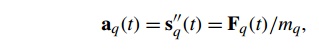
where s^’’_q(t) is the second derivative of the position s_q(t) and F_q(t) is the force on particle q. We also know that the velocity v_q(t) is the first derivative of the position s^’_q(t), so we need to integrate the acceleration to get the velocity, and we need to integrate the velocity to get the position.

We might at first think that we can simply find an antiderivative of the function in Formula 6.3. However, a second look shows us that this approach has problems: the right-hand side contains unknown functions s_q and s_k—not just the variable t—so we’ll instead use a numerical method for estimating the position and the velocity. This means that rather than trying to find simple closed formulas, we’ll approximate

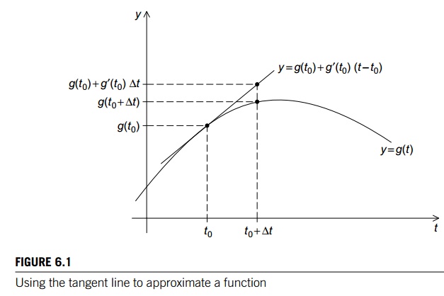
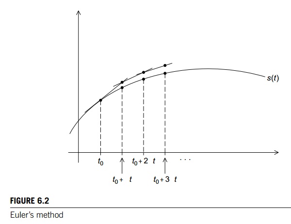
the values of the position and velocity at the times of interest. There are many possible choices for numerical methods, but we’ll use the simplest one: Euler’s method, which is named after the famous Swiss mathematician Leonhard Euler (1707–1783). In Euler’s method, we use the tangent line to approximate a function. The basic idea is that if we know the value of a function g(t₀) at time t₀ and we also know its derivative g^’(t₀) at time t₀, then we can approximate its value at time t₀ + ∆t by using the tangent line to the graph of g(t₀). See Figure 6.1 for an example. Now if we know a point (t0,g(t0)) on a line, and we know the slope of the line g’ (t0), then an equation for line is given by

y = g(t₀) + g’(t₀)(t − t₀).

Since we’re interested in the time t = t₀ + ∆t, we get

g(t + ∆t) ≈ g(t₀) + g’(t₀)(t + ∆t − t) = g(t₀) + ∆tg₀'(t₀).

Note that this formula will work even when g(t) and y are vectors: when this is the case, g^’(t) is also a vector and the formula just adds a vector to a vector multiplied by a scalar, ∆t.

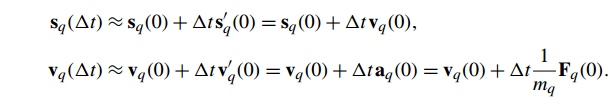
Now we know the value of s_q(t) and s^’_q(t) at time 0, so we can use the tangent line and our formula for the acceleration to compute s_q(∆t) and v_q(∆t):

When we try to extend this approach to the computation of s_q(2∆t) and s^’_q(2∆t), we see that things are a little bit different, since we don’t know the exact value of s_q(∆t)

A struct is also an option. However, if we’re using arrays and we decide to change our program so that it solves three-dimensional problems, in principle, we only need to change the macro DIM. If we try to do this with structs, we’ll need to rewrite the code that accesses individual components of the vector.

For each particle, we need to know the values of

. its mass, 

. its position,

. its velocity, 

. its acceleration, and 

. the total force acting on it. 

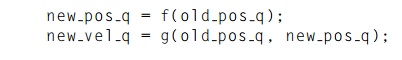
Since we’re using Newtonian physics, the mass of each particle is constant, but the other values will, in general, change as the program proceeds. If we examine our code, we’ll see that once we’ve computed a new value for one of these variables for a given timestep, we never need the old value again. For example, we don’t need to do anything like this

Also, the acceleration is only used to compute the velocity, and its value can be computed in one arithmetic operation from the total force, so we only need to use a local, temporary variable for the acceleration.

For each particle it suffices to store its mass and the current value of its position, velocity, and force. We could store these four variables as a struct and use an array of structs to store the data for all the particles. Of course, there’s no reason that all of the variables associated with a particle need to be grouped together in a struct. We can split the data into separate arrays in a variety of different ways. We’ve chosen to group the mass, position, and velocity into a single struct and store the forces in a separate array. With the forces stored in contiguous memory, we can use a fast function such as memset to quickly assign zeroes to all of the elements at the beginning of each iteration:

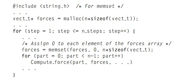
If the force on each particle were a member of a struct, the force members wouldn’t occupy contiguous memory in an array of structs, and we’d have to use a relatively slow for loop to assign zero to each element.

3. Parallelizing the n-body solvers

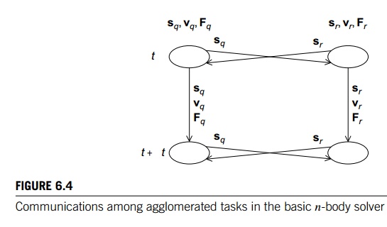
Let’s try to apply Foster’s methodology to the n-body solver. Since we initially want lots of tasks, we can start by making our tasks the computations of the positions, the velocities, and the total forces at each timestep. In the basic algorithm, the algorithm in which the total force on each particle is calculated directly from Formula 6.2, the

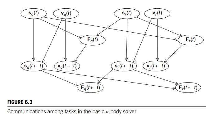
computation of F_q(t), the total force on particle q at time t, requires the positions of each of the particles s_r(t), for each r. The computation of v_q(t + ∆t) requires the velocity at the previous timestep, v_q(t), and the force, F_q(t), at the previous timestep. Finally, the computation of s_q(t + ∆t) requires s_q(t) and v_q(t). The communications among the tasks can be illustrated as shown in Figure 6.3. The figure makes it clear that most of the communication among the tasks occurs among the tasks associated with an individual particle, so if we agglomerate the computations of s_q(t), v_q(t), and F_q(t), our intertask communication is greatly simplified (see Figure 6.4). Now the tasks correspond to the particles and, in the figure, we’ve labeled the communications with the data that’s being communicated. For example, the arrow from particle q at timestep t to particle r at timestep t is labeled with s_q, the position of particle q.

For the reduced algorithm, the “intra-particle” communications are the same. That is, to compute s_q(t + ∆t) we’ll need s_q(t) and v_q(t), and to compute v_q(t + ∆t), we’ll need v_q(t) and F_q(t). Therefore, once again it makes sense to agglomerate the computations associated with a single particle into a composite task.

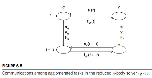
Recollect that in the reduced algorithm, we make use of the fact that the force f_rq = - f_qr. So if q < r, then the communication from task r to task q is the same as in the basic algorithm—in order to compute F_q(t), task/particle q will need s_r(t) from task/particle r. However, the communication from task q to task r is no longer s_q(t), it’s the force on particle q due to particle r, that is, f_qr(t). See Figure 6.5.

The final stage in Foster’s methodology is mapping. If we have n particles and T timesteps, then there will be nT tasks in both the basic and the reduced algorithm. Astrophysical n-body problems typically involve thousands or even millions of par-ticles, so n is likely to be several orders of magnitude greater than the number of available cores. However, T may also be much larger than the number of available cores. So, in principle, we have two “dimensions” to work with when we map tasks to cores. However, if we consider the nature of Euler’s method, we’ll see that attempt-ing to assign tasks associated with a single particle at different timesteps to different cores won’t work very well. Before estimating s_q(t + ∆t) and v_q(t + ∆t), Euler’s method must “know” s_q(t), v_q(t), and a_q(t). Thus, if we assign particle q at time t to core c₀, and we assign particle q at time t + ∆t to core c₁ !=c₀, then we’ll have to communicate s_q(t), v_q(t), and F_q(t) from c₀ to c₁. Of course, if particle q at time t and particle q at time t + ∆t are mapped to the same core, this communication won’t be necessary, so once we’ve mapped the task consisting of the calculations for particle q at the first timestep to core c₀, we may as well map the subsequent computations for particle q to the same cores, since we can’t simultaneously execute the computations for particle q at two different timesteps. Thus, mapping tasks to cores will, in effect, be an assignment of particles to cores.

At first glance, it might seem that any assignment of particles to cores that assigns roughly n=thread count particles to each core will do a good job of balancing the workload among the cores, and for the basic algorithm this is the case. In the basic algorithm the work required to compute the position, velocity, and force is the same for every particle. However, in the reduced algorithm the work required in the forces computation loop is much greater for lower-numbered iterations than the work required for higher-numbered iterations. To see this, recall the pseudocode that computes the total force on particle q in the reduced algorithm:

Then, for example, when q = 0, we’ll make n- 1 passes through the for each particle k > q loop, while when q = n- 1, we won’t make any passes through the loop. Thus, for the reduced algorithm we would expect that a cyclic partition of the particles would do a better job than a block partitition of evenly distributing the computation.

However, in a shared-memory setting, a cyclic partition of the particles among the cores is almost certain to result in a much higher number of cache misses than a block partition, and in a distributed-memory setting, the overhead involved in communicat-ing data that has a cyclic distribution will probably be greater than the overhead involved in communicating data that has a block distribution (see Exercises 6.8 and 6.9).

Therefore with a composite task consisting of all of the computations associated with a single particle throughout the simulation, we conclude the following:

        A block distribution will give the best performance for the basic n-body solver.

        For the reduced n-body solver, a cyclic distribution will best distribute the work-load in the computation of the forces. However, this improved performance may be offset by the cost of reduced cache performance in a shared-memory setting and additional communication overhead in a distributed-memory setting.

In order to make a final determination of the optimal mapping of tasks to cores, we’ll need to do some experimentation.

4. A word about I/O

You may have noticed that our discussion of parallelizing the n-body solver hasn’t touched on the issue of I/O, even though I/O can figure prominently in both of our serial algorithms. We’ve discussed the problem of I/O several times in earlier chap-ters. Recall that different parallel systems vary widely in their I/O capabilities, and with the very basic I/O that is commonly available it is very difficult to obtain high performance. This basic I/O was designed for use by single-process, single-threaded programs, and when multiple processes or multiple threads attempt to access the I/O buffers, the system makes no attempt to schedule their access. For example, if multiple threads attempt to execute

printf("Hello from thread %d of %dnn", my_rank, thread count);

more or less simultaneously, the order in which the output appears will be unpre-dictable. Even worse, one thread’s output may not even appear as a single line. It can happen that the output from one thread appears as multiple segments, and the individual segments are separated by output from other threads.

Thus, as we’ve noted earlier, except for debug output, we generally assume that one process/thread does all the I/O, and when we’re timing program execution, we’ll use the option to only print output for the final timestep. Furthermore, we won’t include this output in the reported run-times.

Of course, even if we’re ignoring the cost of I/O, we can’t ignore its existence. We’ll briefly discuss its implementation when we discuss the details of our parallel implementations.