Transition from Graphical to Algebraic Solution

TRANSITION FROM GRAPHICAL TO ALGEBRAIC SOLUTION

In the graphical method, the solution space is delineated by the half-spaces representing the constraints, and in the simplex method the solution space is represented by m simultaneous linear equations and n nonnegative variables.

We can see visually why the graphical solution space has an infinite number of solution points, but how can we draw a similar conclusion from the algebraic representa-tion of the solution space? The answer is that in the algebraic representation the number of equations m is always less than or equal to the number of variables n.  If m = n, and the equations are consistent, the system has only one solution; but if m < n (which

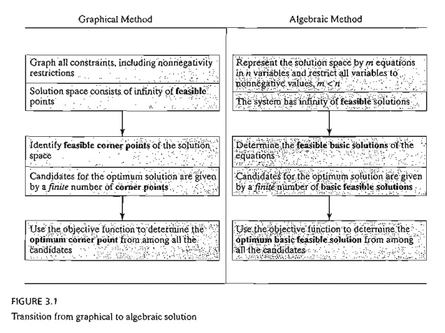
represents the majority of LPs), then the system of equations, again if consistent, will yield an infinite number of solutions. To provide a simple illustration, the equation x = 2 has m = n = 1, and the solution is obviously unique. But, the equation x + y = 1 has m = 1 and n = 2, and it yields an infinite number of solutions (any point on the straight line x + y = 1 is a solution).

Having shown how the LP solution space is represented algebraically, the candi-dates for the optimum (i.e., corner points) are determined from the simultaneous linear equations in the following manner:

Algebraic Determination of Corner Points.

In a set of m X n equations (m < n), if we set n - m variables equal to zero and then solve the m equations for the remaining m variables, the resulting solution, if unique, is called a basic solution and must correspond to a (feasible or infeasible) corner point of the solution space. This means that the maximum number of corner points is

The following example demonstrates the procedure.

Example 3.2-1

Consider the following LP with two variables:

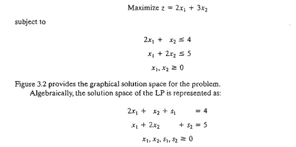
The system has m = 2 equations and n = 4 variables. Thus, according to the given rule, the corner points can be determined algebraically by setting n - m = 4 - 2 =2 variables equal to  zero and then solving for the remaining m = 2 variables. For example, if we set x_l = 0 and x₂ = 0, the equations provide the unique (basic) solution

s_l = 4, s₂ = 5

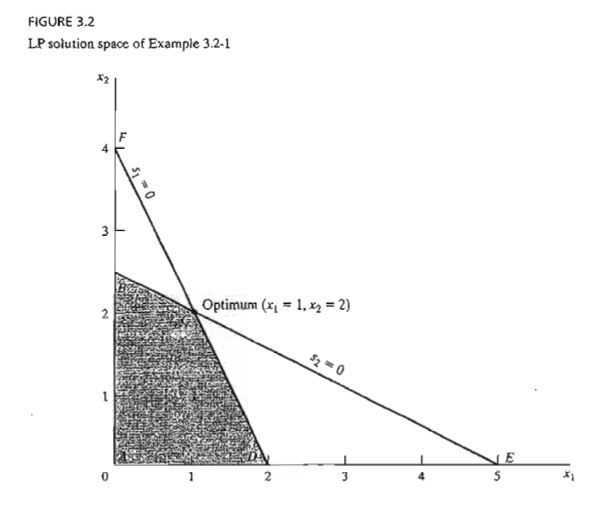
This solution corresponds to point A in Figure 3.2 (convince yourself that s₁ = 4 and s₂ = 5 at point A). Another point can be determined by setting s₁ = 0 and s₂ = 0 and then solving the two equations

2x₁ + x₂ = 4

x₁ + 2x₂ = 5

This yields the basic solution (x_l = 1, x₂  = 2), which is point C in Figure 3.2.

You probably are wondering how one can decide which n - m variables should be set equal to zero to target a specific corner point. Without the benefit of the graphical solution (which is available only for two or three variables), we cannot say which (n - m) zero variables are associated with which corner point. But that does not prevent us from enumerating all the corner points of the solution space. Simply consider all combinations in which n - m variables are set to zero and solve the resulting equations. Once done, the optimum solution is the feasible basic solution (corner point) that yields the best objective value.

In the present example we have  corner points. Looking at Figure 3.2, we can immediately spot the four corner points A, B, C, and D. Where, then, are the remaining two? In fact, points E and F also are corner points for the problem, but they are infeasible because they do not satisfy all the constraints. These infeasible corner points are not candidates for the optimum.

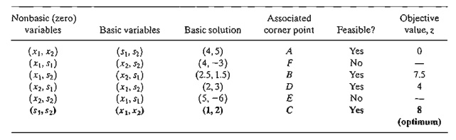
To summarize the transition from the graphical to the algebraic solution, the zero n - m variables are known as nonbasic variables. The remaining m variables are called basic variables and their solution (obtained by solving the m equations) is referred to as basic solution. The following table provides all the basic and nonbasic solutions of the current example.

Remarks. We can see from the computations above that as the problem size increases (that is, m and n become large), the procedure of enumerating all the corner points involves prohibitive computations. For example, for m = 10 and n = 20, it is necessary to solve c²⁰₁₀ = 184,756 sets of 10 X 10 equations, a staggering task indeed, particularly when we realize that a (10 X 20)-LP is a small size in most real-life situations, where hundreds or even thousands of variables and con-straints are not unusual. The simplex method alleviates this computational burden dramatically by investigating only a fraction of all possible basic feasible solutions (corner points) of the solu-tion space. In essence, the simplex method utilizes an intelligent search procedure that locates the optimum corner point in an efficient manner.

PROBLEM SET 3.2A

1. Consider the following LP:

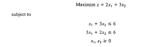
(a) Express the problem in equation form.

(b) Determine all the basic solutions of the problem, and classify them as feasible and infeasible.

*(c) Use direct substitution in the objective function to determine the optimum basic feasible solution.

 (d) Verify graphically that the solution obtained in (c) is the optimum LP solution-hence, conclude that the optimum solution can be determined algebraically by con-sidering the basic feasible solutions only.

*(e) Show how the infeasible basic solutions are represented on the graphical solution space.

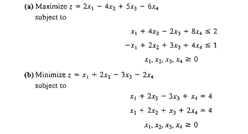
2. Determine the optimum solution for each of the following LPs by enumerating alI the basic solutions.

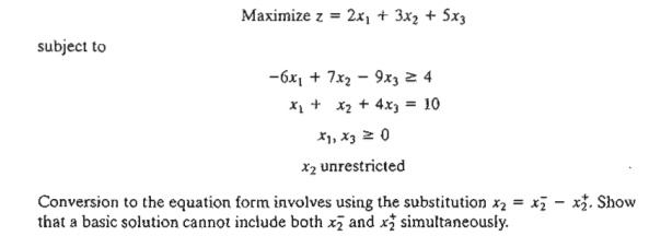
*3.  Show algebraically that all the basic solutions of the following LP are infeasible.

4. Consider the following LP:

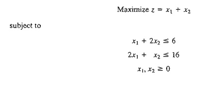
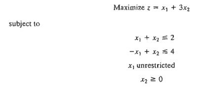
5.       Consider the following LP:

a)     Determine all the basic feasible solutions of the problem.

b)    Use direct substitution in the objective function to determine the best basic solution.

c)     Solve the problem graphically, and verify that the solution obtained in (c) is the optimum.