Theory of Capillary Electrophoresis

Theory of Capillary Electrophoresis

In capillary electrophoresis the sample is injected into a buffered solution retained within a capillary tube. When an electric field is applied to the capillary tube, the sample’s components migrate as the result of two types of mobility: elec- trophoretic mobility and electroosmotic mobility. Electrophoretic mobility is the solute’s response to the applied electric field. As described earlier, cations move toward the negatively charged cathode, anions move toward the positively charged anode, and neutral species, which do not respond to the electric field, re- main stationary. The other contribution to a solute’s migration is electroosmotic flow, which occurs when the buffer solution moves through the capillary in re- sponse to the applied electric field. Under normal conditions the buffer solution moves toward the cathode, sweeping most solutes, even anions, toward the nega- tively charged cathode.

Electrophoretic Mobility 

The velocity with which a solute moves in response to the applied electric field is called its electrophoretic velocity, v_ep; it is defined as

v_ep = μ_epE       ……………..12.35

where μ_ep is the solute’s electrophoretic mobility, and E is the magnitude of the ap- plied electric field. A solute’s electrophoretic mobility is defined as

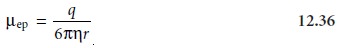
where q is the solute’s charge, μ is the buffer solvent’s viscosity, and r is the solute’s radius. Using equations 12.35 and 12.36, we can make several important conclu- sions about a solute’s electrophoretic velocity. Electrophoretic mobility, and, there- fore, electrophoretic velocity, is largest for more highly charged solutes and solutes of smaller size. Since q is positive for cations and negative for anions, these species migrate in opposite directions. Neutral species, for which q is 0, have an elec- trophoretic velocity of 0.

Electroosmotic Mobility 

When an electric field is applied to a capillary filled with an aqueous buffer, we expect the buffer’s ions to migrate in response to their elec- trophoretic mobility. Because the solvent, H₂O, is neutral, we might reasonably ex- pect it to remain stationary. What is observed under normal conditions, however, is that the buffer solution moves toward the cathode. This phenomenon is called the electroosmotic flow.

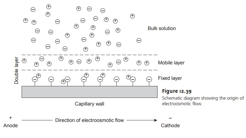
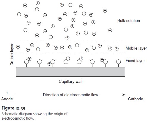
Electroosmosis occurs because the walls of the capillary tubing are electrically charged. The surface of a silica capillary contains large numbers of silanol groups (Si–OH). At pH levels greater than approximately 2 or 3, the silanol groups ionize to form negatively charged silanate ions (Si–O–). Cations from the buffer are at- tracted to the silanate ions. As shown in Figure 12.39, some of these cations bind tightly to the silanate ions, forming an inner, or fixed, layer. Other cations are more loosely bound, forming an outer, or mobile, layer. Together these two layers are called the double layer. Cations in the outer layer migrate toward the cathode. Be- cause these cations are solvated, the solution is also pulled along, producing the electroosmotic flow.

Electroosmotic flow velocity, v_eof, is a function of the magnitude of the applied electric field and the buffer solution’s electroosmotic mobility, μ_eof.

v_eof = μ_eofE       ……………..12.37

Electroosmotic mobility is defined as

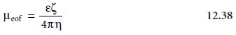
where ε is the buffer solution’s dielectric constant, ξ is the zeta potential, and μ is the buffer solution’s viscosity.

Examining equations 12.37 and 12.38 shows that the zeta potential plays an important role in determining the electroosmotic flow velocity. Two factors deter- mine the zeta potential and, therefore, the electroosmotic velocity. First, the zeta potential is directly proportional to the charge on the capillary walls, with a greater density of silanate ions corresponding to a larger zeta potential. Below a pH of 2, for example, there are few silanate ions; thus, the zeta potential and electroosmotic flow velocity are 0. As the pH level is increased, both the zeta potential and the electroos- motic flow velocity increase. Second, the zeta potential is proportional to the thick- ness of the double layer. Increasing the buffer solution’s ionic strength provides a higher concentration of cations, decreasing the thickness of the double layer.

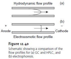
The electroosmotic flow profile is very different from that for a phase moving under forced pressure. Figure 12.40 compares the flow profile for electroosmosis with that for hydrodynamic pressure. The uniform, flat profile for electroosmosis helps to minimize band broadening in capillary elec- trophoresis, thus improving separation efficiency.

Total Mobility

A solute’s net, or total velocity, v, is the sum of its elec- trophoretic velocity and the electroosmotic flow velocity; thus,

vtot = vep + veof

μtot = μep + μeof

Under normal conditions the following relationships hold

(vtot)cations > veof

(vtot)anions < veof

(vtot)neutrals = veof

Thus, cations elute first in an order corresponding to their electrophoretic mobili- ties, with small, highly charged cations eluting before larger cations of lower charge. Neutral species elute as a single band, with an elution rate corresponding to the electroosmotic flow velocity. Finally, anions are the last components to elute, with smaller, highly charged anions having the longest elution time.

Migration Time 

A solute’s total velocity is given by

where l is the distance the solute travels between its point of injection and the detec- tor, and t_m is the migration time. Since

vtot = μtotE = (μep + μeof)E

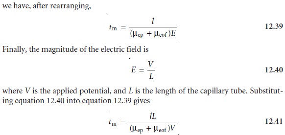
Examining equation 12.41 shows that we can decrease a solute’s migration time (and thus the total analysis time) by applying a higher voltage or by using a shorter capillary tube. Increasing the electroosmotic flow also shortens the analysis time, but, as we will see shortly, at the expense of resolution.

Efficiency 

The efficiency of capillary electrophoresis is characterized by the num- ber of theoretical plates, N, just as it is in GC or HPLC. In capillary electrophoresis, the number of theoretic plates is determined by

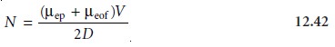
where D is the solute’s diffusion coefficient. From equation 12.42 it is easy to see that the efficiency of a capillary electrophoretic separation increases with higher voltages. Again, increasing the electroosmotic flow velocity improves efficiency, but at the expense of resolution. Two additional observations deserve comment.

First, solutes with larger electrophoretic mobilities (in the same direction as the electroosmotic flow) have greater efficiencies; thus, smaller, more highly charged solutes are not only the first solutes to elute, but do so with greater efficiency. Sec- ond, efficiency in capillary electrophoresis is independent of the capillary’s length. Typical theoretical plate counts are approximately 100,000–200,000 for capillary electrophoresis.

Selectivity 

In chromatography, selectivity is defined as the ratio of the capacity factors for two solutes (equation 12.11). In capillary electrophoresis, the analogous expression for selectivity is

where μ_ep,1 and μ_ep,2 are the electrophoretic mobilities for solutes 1 and 2, respec- tively, chosen such that α >= 1. Selectivity often can be improved by adjusting the pH of the buffer solution. For example, NH₄+ is a weak acid with a pK of 9.24. At a pH of 9.24 the concentrations of NH₄+ and NH are equal. Decreasing the pH below9.24 increases its electrophoretic mobility because a greater fraction of the solute is present as the cation NH₄+. On the other hand, raising the pH above 9.24 increases the proportion of the neutral NH₃, decreasing its electrophoretic mobility.

Resolution 

The resolution between two solutes is

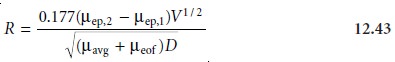
where μ_avg is the average electrophoretic mobility for the two solutes. Examining equation 12.43 shows that increasing the applied voltage and decreasing the elec- troosmotic flow velocity improves resolution. The latter effect is particularly impor- tant because increasing electroosmotic flow improves analysis time and efficiency while decreasing resolution.