The Trapezoidal Rule in MPI

THE TRAPEZOIDAL RULE IN MPI

Printing messages from processes is all well and good, but we’re probably not tak-ing the trouble to learn to write MPI programs just to print messages. Let’s take a look at a somewhat more useful program—let’s write a program that implements the trapezoidal rule for numerical integration.

1. The trapezoidal rule

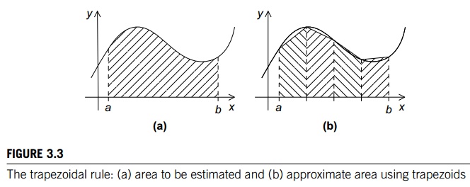
Recall that we can use the trapezoidal rule to approximate the area between the graph of a function, y = f(x), two vertical lines, and the x-axis. See Figure 3.3. The basic idea is to divide the interval on the x-axis into n equal subintervals. 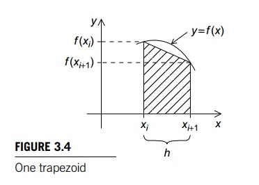Then we approxi-mate the area lying between the graph and each subinterval by a trapezoid whose base is the subinterval, whose vertical sides are the vertical lines through the endpoints of the subinterval, and whose fourth side is the secant line joining the points where the vertical lines cross the graph. See Figure 3.4. 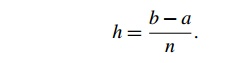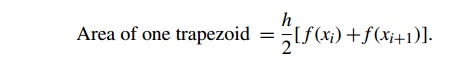If the endpoints of the subinterval are x_i and x_i+1, then the length of the subinterval is h = x_i+1- x_i. Also, if the lengths of the two vertical segments are f(x_i) and f (x_i+1), then the area of the trapezoid is

Since we chose the n subintervals so that they would all have the same length, we also know that if the vertical lines bounding the region are x = a and x = b, then

Thus, if we call the leftmost endpoint x₀, and the rightmost endpoint x_n, we have

x₀ = a, x₁ = a + h, x₂ = a + 2h, …., x_n -₁ = a + (n-1)h, x_n = b,

and the sum of the areas of the trapezoids—our approximation to the total area—is

Sum of trapezoid areas = h[ f (x₀)/2 +  f (x₁) + f (x₂) +   + f (x_n-₁)+  f (x_n)/2].

Thus, pseudo-code for a serial program might look something like this:

/* Input: a, b, n */

 h = (b-a)/n;

approx = (f(a) + f(b))/2.0;

for (i = 1; i <= n-1; i++) {

x_i = a + i* h;

 approx += f(x_i);

}

approx = h*approx;

2. Parallelizing the trapezoidal rule

It is not the most attractive word, but, as we noted in Chapter 1, people who write parallel programs do use the verb “parallelize” to describe the process of converting a serial program or algorithm into a parallel program.

Recall that we can design a parallel program using four basic steps:

        Partition the problem solution into tasks.

        Identify the communication channels between the tasks.

        Aggregate the tasks into composite tasks.

        Map the composite tasks to cores.

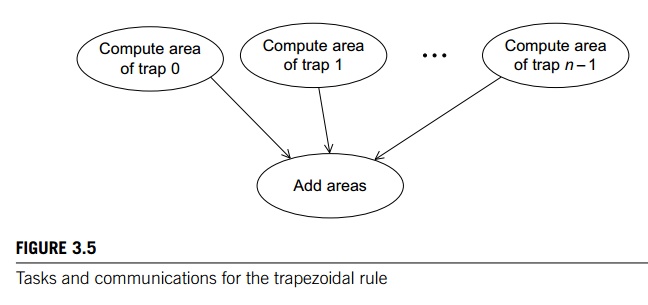
In the partitioning phase, we usually try to identify as many tasks as possible. For the trapezoidal rule, we might identify two types of tasks: one type is finding the area of a single trapezoid, and the other is computing the sum of these areas. Then the communication channels will join each of the tasks of the first type to the single task of the second type. See Figure 3.5.

So how can we aggregate the tasks and map them to the cores? Our intuition tells us that the more trapezoids we use, the more accurate our estimate will be. That is, we should use many trapezoids, and we will use many more trapezoids than cores. Thus, we need to aggregate the computation of the areas of the trapezoids into groups. A natural way to do this is to split the interval [a, b] up into comm sz subintervals. If comm sz evenly divides n, the number of trapezoids, we can simply apply the trape-zoidal rule with n=comm sz trapezoids to each of the comm sz subintervals. To finish, we can have one of the processes, say process 0, add the estimates.

Let’s make the simplifying assumption that comm sz evenly divides n. Then pseudo-code for the program might look something like the following:

1        Get a, b, n;

2        h = (b a)/n;

3        local_n = n/comm sz;

4        local_a        =       a + my rank*local_n*h;

5        local_b        =       local_a + local_n*h;

 6         Local_integral = Trap(local_a, local_b, local_n, h);

7        if (my_rank != 0)

8        Send local_integral to process 0;

9        else /*  my rank == 0  */

10      total_integral = local_integral;

11      for (proc = 1; proc < comm._sz; proc++) {

          Receive local_integral from proc;

          total_integral += local_integral;

          }

          }

          if (my_rank == 0)

          print result;

Let’s defer, for the moment, the issue of input and just “hardwire” the values for a, b, and n. When we do this, we get the MPI program shown in Program 3.2. The Trap function is just an implementation of the serial trapezoidal rule. See Program 3.3.

Notice that in our choice of identifiers, we try to differentiate between local and global variables. Local variables are variables whose contents are significant only on the process that’s using them. Some examples from the trapezoidal rule program are local_a, local_b, and local_n. Variables whose contents are significant to all the processes are sometimes called global variables. Some examples from the trapezoidal rule are a, b, and n. Note that this usage is different from the usage you learned in your introductory programming class, where local variables are private to a single function and global variables are accessible to all the functions. However, no confusion should arise, since the context will usually make the meaning clear.