The Analysis Framework

The Analysis Framework

1. Measuring an Input’s Size

2. Units for Measuring Running Time

3. Orders of Growth

4. Worst-Case, Best-Case, and Average-Case Efficiencies

5. Recapitulation of the Analysis Framework

In this section, we outline a general framework for analyzing the efficiency of algo-rithms. We already mentioned in Section 1.2 that there are two kinds of efficiency: time efficiency and space efficiency. Time efficiency, also called time complexity, indicates how fast an algorithm in question runs. Space efficiency, also called space complexity, refers to the amount of memory units required by the algorithm in ad-dition to the space needed for its input and output. In the early days of electronic computing, both resources—time and space—were at a premium. Half a century of relentless technological innovations have improved the computer’s speed and memory size by many orders of magnitude. Now the amount of extra space re-quired by an algorithm is typically not of as much concern, with the caveat that there is still, of course, a difference between the fast main memory, the slower secondary memory, and the cache. The time issue has not diminished quite to the same extent, however. In addition, the research experience has shown that for most problems, we can achieve much more spectacular progress in speed than in space. Therefore, following a well-established tradition of algorithm textbooks, we primarily concentrate on time efficiency, but the analytical framework introduced here is applicable to analyzing space efficiency as well.

Measuring an Input’s Size

Let’s start with the obvious observation that almost all algorithms run longer on larger inputs. For example, it takes longer to sort larger arrays, multiply larger matrices, and so on. Therefore, it is logical to investigate an algorithm’s efficiency as a function of some parameter n indicating the algorithm’s input size.¹ In most cases, selecting such a parameter is quite straightforward. For example, it will be the size of the list for problems of sorting, searching, finding the list’s smallest element, and most other problems dealing with lists. For the problem of evaluating a polynomial p(x) = a_nxⁿ + ^{. . .} + a₀ of degree n, it will be the polynomial’s degree or the number of its coefficients, which is larger by 1 than its degree. You’ll see from the discussion that such a minor difference is inconsequential for the efficiency analysis.

There are situations, of course, where the choice of a parameter indicating an input size does matter. One such example is computing the product of two n × n matrices. There are two natural measures of size for this problem. The first and more frequently used is the matrix order n. But the other natural contender is the total number of elements N in the matrices being multiplied. (The latter is also more general since it is applicable to matrices that are not necessarily square.) Since there is a simple formula relating these two measures, we can easily switch from one to the other, but the answer about an algorithm’s efficiency will be qualitatively different depending on which of these two measures we use (see Problem 2 in this section’s exercises).

The choice of an appropriate size metric can be influenced by operations of the algorithm in question. For example, how should we measure an input’s size for a spell-checking algorithm? If the algorithm examines individual characters of its input, we should measure the size by the number of characters; if it works by processing words, we should count their number in the input.

We should make a special note about measuring input size for algorithms solving problems such as checking primality of a positive integer n. Here, the input is just one number, and it is this number’s magnitude that determines the input size. In such situations, it is preferable to measure size by the number b of bits in the n’s binary representation:

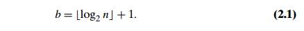
This metric usually gives a better idea about the efficiency of algorithms in question.

Units for Measuring Running Time

The next issue concerns units for measuring an algorithm’s running time. Of course, we can simply use some standard unit of time measurement—a second, or millisecond, and so on—to measure the running time of a program implement-ing the algorithm. There are obvious drawbacks to such an approach, however: dependence on the speed of a particular computer, dependence on the quality of a program implementing the algorithm and of the compiler used in generating the machine code, and the difficulty of clocking the actual running time of the pro-gram. Since we are after a measure of an algorithm’s efficiency, we would like to have a metric that does not depend on these extraneous factors.

One possible approach is to count the number of times each of the algorithm’s operations is executed. This approach is both excessively difficult and, as we shall see, usually unnecessary. The thing to do is to identify the most important operation of the algorithm, called the basic operation, the operation contributing the most to the total running time, and compute the number of times the basic operation is executed.

As a rule, it is not difficult to identify the basic operation of an algorithm: it is usually the most time-consuming operation in the algorithm’s innermost loop. For example, most sorting algorithms work by comparing elements (keys) of a list being sorted with each other; for such algorithms, the basic operation is a key comparison. As another example, algorithms for mathematical problems typically involve some or all of the four arithmetical operations: addition, subtraction, multiplication, and division. Of the four, the most time-consuming operation is division, followed by multiplication and then addition and subtraction, with the last two usually considered together.²

Thus, the established framework for the analysis of an algorithm’s time ef-ficiency suggests measuring it by counting the number of times the algorithm’s basic operation is executed on inputs of size n. We will find out how to compute such a count for nonrecursive and recursive algorithms in Sections 2.3 and 2.4, respectively.

Here is an important application. Let c_op be the execution time of an algo-rithm’s basic operation on a particular computer, and let C(n) be the number of times this operation needs to be executed for this algorithm. Then we can estimate the running time T (n) of a program implementing this algorithm on that computer by the formula

T (n) ≈ c_opC(n).

Of course, this formula should be used with caution. The count C(n) does not contain any information about operations that are not basic, and, in fact, the count itself is often computed only approximately. Further, the constant c_op is also an approximation whose reliability is not always easy to assess. Still, unless n is extremely large or very small, the formula can give a reasonable estimate of the algorithm’s running time. It also makes it possible to answer such questions as “How much faster would this algorithm run on a machine that is 10 times faster than the one we have?” The answer is, obviously, 10 times. Or, assuming that C(n) = ₂¹ n(n − 1), how much longer will the algorithm run if we double its input size? The answer is about four times longer. Indeed, for all but very small values of n.

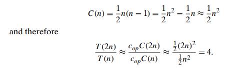
Note that we were able to answer the last question without actually knowing the value of c_op: it was neatly cancelled out in the ratio. Also note that ₂¹ , the multiplicative constant in the formula for the count C(n), was also cancelled out. It is for these reasons that the efficiency analysis framework ignores multiplicative constants and concentrates on the count’s order of growth to within a constant multiple for large-size inputs.

Orders of Growth

Why this emphasis on the count’s order of growth for large input sizes? A differ-ence in running times on small inputs is not what really distinguishes efficient algorithms from inefficient ones. When we have to compute, for example, the greatest common divisor of two small numbers, it is not immediately clear how much more efficient Euclid’s algorithm is compared to the other two algorithms discussed in Section 1.1 or even why we should care which of them is faster and by how much. 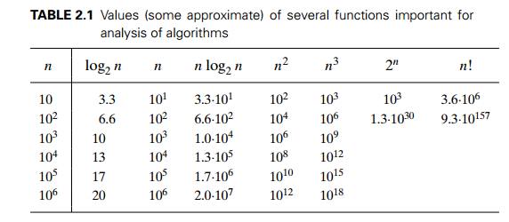It is only when we have to find the greatest common divisor of two large numbers that the difference in algorithm efficiencies becomes both clear and important. For large values of n, it is the function’s order of growth that counts: just look at Table 2.1, which contains values of a few functions particularly important for analysis of algorithms.

The magnitude of the numbers in Table 2.1 has a profound significance for the analysis of algorithms. The function growing the slowest among these is the logarithmic function. It grows so slowly, in fact, that we should expect a program

implementing an algorithm with a logarithmic basic-operation count to run practi-cally instantaneously on inputs of all realistic sizes. Also note that although specific values of such a count depend, of course, on the logarithm’s base, the formula

log_a n = log_a b log_b n

makes it possible to switch from one base to another, leaving the count logarithmic but with a new multiplicative constant. This is why we omit a logarithm’s base and write simply log n in situations where we are interested just in a function’s order of growth to within a multiplicative constant.

On the other end of the spectrum are the exponential function 2ⁿ and the factorial function n! Both these functions grow so fast that their values become astronomically large even for rather small values of n. (This is the reason why we did not include their values for n > 10² in Table 2.1.) For example, it would take about 4 ^. 10¹⁰ years for a computer making a trillion (10 ¹²) operations per second to execute 2¹⁰⁰ operations. Though this is incomparably faster than it would have taken to execute 100! operations, it is still longer than 4.5 billion (4.5 ^. 10⁹) years— the estimated age of the planet Earth. There is a tremendous difference between the orders of growth of the functions 2ⁿ and n!, yet both are often referred to as “exponential-growth functions” (or simply “exponential”) despite the fact that, strictly speaking, only the former should be referred to as such. The bottom line, which is important to remember, is this:

Algorithms that require an exponential number of operations are practical for solving only problems of very small sizes.

Another way to appreciate the qualitative difference among the orders of growth of the functions in Table 2.1 is to consider how they react to, say, a twofold increase in the value of their argument n. The function log₂ n increases in value by just 1 (because log₂ 2n = log ₂ 2 + log₂ n = 1 + log₂ n); the linear function increases twofold, the linearithmic function n log₂ n increases slightly more than twofold; the quadratic function n² and cubic function n³ increase fourfold and eightfold, respectively (because (2n)² = 4n² and (2n)³ = 8n³); the value of 2ⁿ gets squared (because 2²ⁿ = (2ⁿ)²); and n! increases much more than that (yes, even mathematics refuses to cooperate to give a neat answer for n!).

Worst-Case, Best-Case, and Average-Case Efficiencies

In the beginning of this section, we established that it is reasonable to measure an algorithm’s efficiency as a function of a parameter indicating the size of the algorithm’s input. But there are many algorithms for which running time depends not only on an input size but also on the specifics of a particular input. Consider, as an example, sequential search. This is a straightforward algorithm that searches for a given item (some search key K) in a list of n elements by checking successive elements of the list until either a match with the search key is found or the list is exhausted. Here is the algorithm’s pseudocode, in which, for simplicity, a list is implemented as an array. It also assumes that the second condition A[i]  = K will not be checked if the first one, which checks that the array’s index does not exceed its upper bound, fails.

ALGORITHM    

SequentialSearch(A[0..n − 1], K)

//Searches for a given value in a given array by sequential search //Input: An array A[0..n − 1] and a search key K

//Output: The index of the first element in A that matches K

                                        or −1 if there are no matching elements

i ← 0

while i < n and A[i]  = K do i ← i + 1

if i < n return i else return −1

Clearly, the running time of this algorithm can be quite different for the same list size n. In the worst case, when there are no matching elements or the first matching element happens to be the last one on the list, the algorithm makes the largest number of key comparisons among all possible inputs of size

n: C_worst (n) = n.

The worst-case efficiency of an algorithm is its efficiency for the worst-case input of size n, which is an input (or inputs) of size n for which the algorithm runs the longest among all possible inputs of that size. The way to determine the worst-case efficiency of an algorithm is, in principle, quite straightforward: analyze the algorithm to see what kind of inputs yield the largest value of the basic operation’s count C(n) among all possible inputs of size n and then compute this

worst-case value C_worst (n). (For sequential search, the answer was obvious. The methods for handling less trivial situations are explained in subsequent sections of

this chapter.) Clearly, the worst-case analysis provides very important information about an algorithm’s efficiency by bounding its running time from above. In other words, it guarantees that for any instance of size n, the running time will not exceed

C_worst (n), its running time on the worst-case inputs.

The best-case efficiency of an algorithm is its efficiency for the best-case input of size n, which is an input (or inputs) of size n for which the algorithm runs the fastest among all possible inputs of that size. Accordingly, we can analyze the best-case efficiency as follows. First, we determine the kind of inputs for which the count C(n) will be the smallest among all possible inputs of size n. (Note that the best case does not mean the smallest input; it means the input of size n for which the algorithm runs the fastest.) Then we ascertain the value of C(n) on these most convenient inputs. For example, the best-case inputs for sequential search are lists

of size n with their first element equal to a search key; accordingly, C_best (n) = 1 for this algorithm.

The analysis of the best-case efficiency is not nearly as important as that of the worst-case efficiency. But it is not completely useless, either. Though we should not expect to get best-case inputs, we might be able to take advantage of the fact that for some algorithms a good best-case performance extends to some useful types of inputs close to being the best-case ones. For example, there is a sorting algorithm (insertion sort) for which the best-case inputs are already sorted arrays on which the algorithm works very fast. Moreover, the best-case efficiency deteriorates only slightly for almost-sorted arrays. Therefore, such an algorithm might well be the method of choice for applications dealing with almost-sorted arrays. And, of course, if the best-case efficiency of an algorithm is unsatisfactory, we can immediately discard it without further analysis.

It should be clear from our discussion, however, that neither the worst-case analysis nor its best-case counterpart yields the necessary information about an algorithm’s behavior on a “typical” or “random” input. This is the information that the average-case efficiency seeks to provide. To analyze the algorithm’s average-case efficiency, we must make some assumptions about possible inputs of size n.

Let’s consider again sequential search. The standard assumptions are that

(a) the probability of a successful search is equal to p (0 ≤ p ≤ 1) and (b) the probability of the first match occurring in the ith position of the list is the same for every i. Under these assumptions—the validity of which is usually difficult to verify, their reasonableness notwithstanding—we can find the average number of key comparisons C_avg(n) as follows. In the case of a successful search, the probability of the first match occurring in the ith position of the list is p/n for every i, and the number of comparisons made by the algorithm in such a situation is obviously i. In the case of an unsuccessful search, the number of comparisons will be n with the probability of such a search being (1 − p). Therefore,

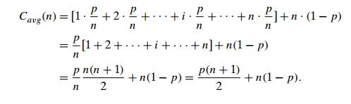
This general formula yields some quite reasonable answers. For example, if p = 1 (the search must be successful), the average number of key comparisons made by sequential search is (n + 1)/2; that is, the algorithm will inspect, on average, about half of the list’s elements. If p = 0 (the search must be unsuccessful), the average number of key comparisons will be n because the algorithm will inspect all n elements on all such inputs.

As you can see from this very elementary example, investigation of the average-case efficiency is considerably more difficult than investigation of the worst-case and best-case efficiencies. The direct approach for doing this involves dividing all instances of size n into several classes so that for each instance of the class the number of times the algorithm’s basic operation is executed is the same. (What were these classes for sequential search?) Then a probability distribution of inputs is obtained or assumed so that the expected value of the basic operation’s count can be found.

The technical implementation of this plan is rarely easy, however, and prob-abilistic assumptions underlying it in each particular case are usually difficult to verify. Given our quest for simplicity, we will mostly quote known results about the average-case efficiency of algorithms under discussion. If you are interested in derivations of these results, consult such books as [Baa00], [Sed96], [KnuI], [KnuII], and [KnuIII].

It should be clear from the preceding discussion that the average-case ef-ficiency cannot be obtained by taking the average of the worst-case and the best-case efficiencies. Even though this average does occasionally coincide with the average-case cost, it is not a legitimate way of performing the average-case analysis.

Does one really need the average-case efficiency information? The answer is unequivocally yes: there are many important algorithms for which the average-case efficiency is much better than the overly pessimistic worst-case efficiency would lead us to believe. So, without the average-case analysis, computer scientists could have missed many important algorithms.

Yet another type of efficiency is called amortized efficiency. It applies not to a single run of an algorithm but rather to a sequence of operations performed on the same data structure. It turns out that in some situations a single operation can be expensive, but the total time for an entire sequence of n such operations is always significantly better than the worst-case efficiency of that single operation multiplied by n. So we can “amortize” the high cost of such a worst-case occur-rence over the entire sequence in a manner similar to the way a business would amortize the cost of an expensive item over the years of the item’s productive life. This sophisticated approach was discovered by the American computer scientist Robert Tarjan, who used it, among other applications, in developing an interest-ing variation of the classic binary search tree (see [Tar87] for a quite readable nontechnical discussion and [Tar85] for a technical account). We will see an ex-ample of the usefulness of amortized efficiency in Section 9.2, when we consider algorithms for finding unions of disjoint sets.

Recapitulation of the Analysis Framework

Before we leave this section, let us summarize the main points of the framework outlined above.

Both time and space efficiencies are measured as functions of the algorithm’s input size.

Time efficiency is measured by counting the number of times the algorithm’s basic operation is executed. Space efficiency is measured by counting the number of extra memory units consumed by the algorithm.

The efficiencies of some algorithms may differ significantly for inputs of the same size. For such algorithms, we need to distinguish between the worst-case, average-case, and best-case efficiencies.

The framework’s primary interest lies in the order of growth of the algorithm’s running time (extra memory units consumed) as its input size goes to infinity.

In the next section, we look at formal means to investigate orders of growth. In Sections 2.3 and 2.4, we discuss particular methods for investigating nonrecursive and recursive algorithms, respectively. It is there that you will see how the analysis framework outlined here can be applied to investigating the efficiency of specific algorithms. You will encounter many more examples throughout the rest of the book.

Exercises 2.1

                                                                    For each of the following algorithms, indicate (i) a natural size metric for its inputs, (ii) its basic operation, and (iii) whether the basic operation count can be different for inputs of the same size:

                                                                            computing the sum of n numbers

                                                                            computing n!

                                                                            finding the largest element in a list of n numbers

                                                                            Euclid’s algorithm

                                                                            sieve of Eratosthenes

                                                                            pen-and-pencil algorithm for multiplying two n-digit decimal integers

                                                                    a. Consider the definition-based algorithm for adding two n × n matrices. What is its basic operation? How many times is it performed as a function of the matrix order n? As a function of the total number of elements in the input matrices?

                                                                    Answer the same questions for the definition-based algorithm for matrix multiplication.

         Consider a variation of sequential search that scans a list to return the number of occurrences of a given search key in the list. Does its efficiency differ from the efficiency of classic sequential search?

         a. Glove selection There are 22 gloves in a drawer: 5 pairs of red gloves, 4 pairs of yellow, and 2 pairs of green. You select the gloves in the dark and can check them only after a selection has been made. What is the smallest number of gloves you need to select to have at least one matching pair in the best case? In the worst case?

                  Missing socks Imagine that after washing 5 distinct pairs of socks, you discover that two socks are missing. Of course, you would like to have the largest number of complete pairs remaining. Thus, you are left with 4 complete pairs in the best-case scenario and with 3 complete pairs in the worst case. Assuming that the probability of disappearance for each of the 10 socks is the same, find the probability of the best-case scenario; the probability of the worst-case scenario; the number of pairs you should expect in the average case.

         a. Prove formula (2.1) for the number of bits in the binary representation of a positive decimal integer.

                  Prove the alternative formula for the number of bits in the binary repre-sentation of a positive integer n:

b =  log₂(n + 1) .

c.  What would be the analogous formulas for the number of decimal digits?

d.   Explain why, within the accepted analysis framework, it does not matter whether we use binary or decimal digits in measuring n’s size.

6.       Suggest how any sorting algorithm can be augmented in a way to make the best-case count of its key comparisons equal to just n − 1 (n is a list’s size, of course). Do you think it would be a worthwhile addition to any sorting algorithm?

7.       Gaussian elimination, the classic algorithm for solving systems of n linear equations in n unknowns, requires about ₃¹ n³ multiplications, which is the algorithm’s basic operation.

a.    How much longer should you expect Gaussian elimination to work on a system of 1000 equations versus a system of 500 equations?

b.   You are considering buying a computer that is 1000 times faster than the one you currently have. By what factor will the faster computer increase the sizes of systems solvable in the same amount of time as on the old computer?

8. For each of the following functions, indicate how much the function’s value will change if its argument is increased fourfold.

9. For each of the following pairs of functions, indicate whether the first function of each of the following pairs has a lower, same, or higher order of growth (to within a constant multiple) than the second function.

10. Invention of chess

According to a well-known legend, the game of chess was invented many centuries ago in northwestern India by a certain sage. When he took his invention to his king, the king liked the game so much that he offered the inventor any reward he wanted. The inventor asked for some grain to be obtained as follows: just a single grain of wheat was to be placed on the first square of the chessboard, two on the second, four on the third, eight on the fourth, and so on, until all 64 squares had been filled. If it took just 1 second to count each grain, how long would it take to count all the grain due to him?

How long would it take if instead of doubling the number of grains for each square of the chessboard, the inventor asked for adding two grains?