Symbolic Analysis

Symbolic Analysis

1 Affine Expressions of Reference Variables

2 Data-Flow Problem Formulation

3 Region-Based Symbolic Analysis

4 Exercises for Section 9.8

9.9 Summary of Chapter 9

We shall use symbolic analysis in this section to illustrate the use of region-based analysis. In this analysis, we track the values of variables in programs symbolically as expressions of input variables and other variables, which we call reference variables. Expressing variables in terms of the same set of ref-erence variables draws out their relationships. Symbolic analysis can be used for a range of purposes such as optimization, parallelization, and analyses for program understanding.

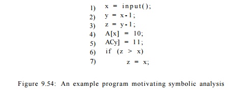
Example 9 . 5 6 :  Consider the simple example program in Fig. 9.54.  Here, we use x as the sole reference variable. Symbolic analysis will find that y has the value x — 1 and z has the value x — 2 after their respective assignment statements in lines (2) and (3).  This information is useful, for example, in determining that the two assignments in lines (4) and (5) write to different memory locations and can thus be executed in parallel.  Furthermore, we can tell that the condition z  >  x  is never true, thus  allowing the  optimizer to remove the  conditional statement in lines (6) and (7) all together.

1. Affine Expressions of Reference Variables

Since we cannot create succinct and closed-form symbolic expressions for all values computed, we choose an abstract domain and approximate the compu-tations with the most precise expressions within the domain. We have already seen an example of this strategy before: constant propagation. In constant propagation, our abstract domain consists of the constants, an UNDEF symbol if we have not yet determined if the value is a constant, and a special NAC symbol that is used whenever a variable is found not to be a constant.

The symbolic analysis we present here expresses values as affine expressions of reference variables whenever possible. An expression is affine with respect to variables i > 2 , . . .  ,vn    if it can be expressed as Co + c1V1 + • • • + cnvn, where  are constants. Such expressions are informally known as linear expressions. Strictly speaking, an affine expression is linear only if CQ is zero. We are interested in affine expressions because they are often used to index arrays in loops—such information is useful for optimizations and parallelization. Much more will be said about this topic in Chapter 11.

Induction  Variables

Instead of using program variables as reference variables, an affine expression can also be written in terms of the count of iterations through the loop. Vari-ables whose values can be expressed as cii + c 0 , where i is the count of iterations through  the  closest  enclosing loop, are known  as  induction  variables.

Example 9 . 5 7 :  Consider the code fragment

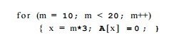
Suppose we introduce for the loop a variable, say i, representing the number of iterations executed. The value i is 0 in the first iteration of the loop, 1 in the second, and so on. We can express variable m as an affine expression of i, namely m — i + 10. Variable x, which is 3m, takes on values 30,33,... ,57 during successive iterations of the loop. Thus, x has the affine expression x = 30 + Si.

We conclude that both m and x are induction variables of this loop.    •

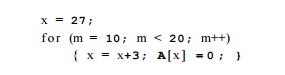
Expressing variables as affine expressions of loop indexes makes the series of values being computed explicit and enables several transformations. The series of values taken on by an induction variable can be computed with additions rather than multiplications.  This transformation is known as  "strength reduction" and was introduced in Sections 8.7 and 9.1. For instance, we can eliminate the multiplication x=m*3 from the loop of Example 9.57 by rewriting the loop as

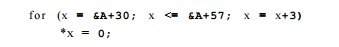
In addition, notice that the locations assigned 0 in that loop, SzA + S0, &,A + 33,... , & A + 57, are also affine expressions of the loop index. In fact, this series of integers is the only one that needs to be computed; We need neither m nor x. The code above can be replaced simply by:

Besides speeding up the computation, symbolic analysis is also useful for parallelization. When the array indexes in a loop are affine expressions of loop indexes, we can reason about relations of data accessed across the iterations. For example, we can tell that the locations written are different in each itera-tion and therefore all the iterations in the loop can be executed in parallel on different processors. Such information is used in Chapters 10 and 11 to extract parallelism from sequential programs.

Other  Reference Variables

If a variable is not a linear function of the reference variables already chosen, we have the option of treating its value as reference for future operations.  For example, consider the code fragment:

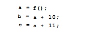
While the  value  held  by  a  after  the function  call cannot  itself be  expressed as a linear function of any reference variables, it can be used as reference for subsequent statements. For example, using a as a reference variable, we can discover that c is one larger than b at the end of the program.

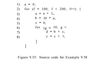
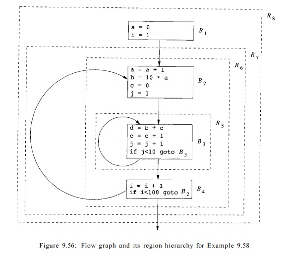
Example 9 . 5 8 : Our running example for this section is based on the source code shown in Fig. 9.55. The inner and outer loops are easy to understand, since / and g are not modified except as required by the for-loops. It is thus possible to replace / and g by reference variables i and j that count the number of        iterations    of the outer and    inner loops,  respectively.          That is,  we can let /       —  i + 99    and g =  j + 9,       and substitute for  /  and         g throughout. When translating to intermediate code, we can take advantage of the fact that each loop iterates at least once, and so postpone the test for i < 100 and j < 10 to the ends of the loops. Figure 9.56 shows the flow graph for the code of Fig. 9.55, after introducing i and j and treating the for-loops as if they were repeat-loops.

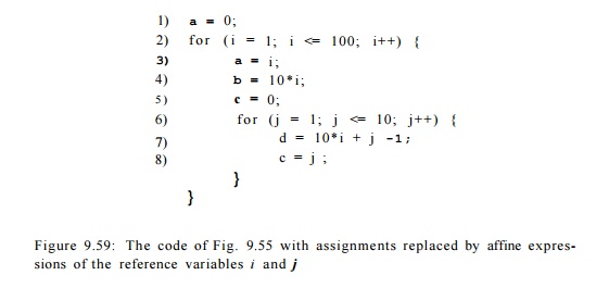
It turns out that a, b, c, and d are all induction variables. The sequences of values assigned to the variables in each line of the code are shown in Figure 9.57. As we shall see, it is possible to discover the affine expressions for these variables, in terms of the reference variables i and j.  That is, at line (4) a — i, at line (7)  d = lOi + j — 1, and at line (8), c = j.  

2. Data-Flow Problem Formulation

This analysis finds affine expressions of reference variables introduced (1) to count the number of iterations executed in each loop, and (2) to hold values at the entry of regions where necessary. This analysis also finds induction variables, loop invariants, as well as constants, as degenerate affine expressions. Note that this analysis cannot find all constants because it only tracks affine expressions of reference variables.

Data - Flow Values : Symbolic  Maps

The domain of data-flow values for this analysis is symbolic maps, which are functions that map each variable in the program to a value. The value is either an affine function of reference values, or the special symbol NAA to represent a non-afflne expression. If there is only one variable, the bottom value of the semilattice is a map that sends the variable to NAA. The semilattice for n variables is simply the product of the individual semilattices. We use m N A A to denote the bottom of the semilattice which maps all variables to NAA . We can define the symbolic map that sends all variables to an unknown value to be the top data-flow value, as we did for constant propagation. However, we do not need top values in region-based analysis.

Example 9 . 5 9 : The symbolic maps associated with each block for the code in Example 9.58 are shown in Figure 9.58.  We shall see later how these maps are discovered; they are the result of doing region-based data-flow analysis on the flow graph of Fig. 9.56.

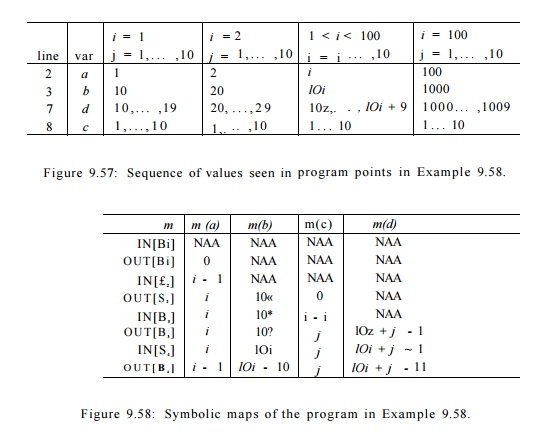
Figure 9.58:  Symbolic maps of the program in Example 9.58.

The symbolic map associated with the entry of the program is m N A A .  At the exit of Bi, the value of a is set to 0.  Upon entry to block _B2, a has value 0 in the first iteration and increments by one in each subsequent iteration of the outer loop. Thus a has value i — 1 at the entry of the ith iteration and value i at the end. The symbolic map at the entry of B2 maps variables 6, c, d to NAA, because the variables have unknown values on entry to the inner loop. Their values depend on the number of iterations of the outer loop, so far. The symbolic map on exit from B2 reflects the assignment statements to a, b, and c in that block. The rest of the symbolic maps can be deduced in a similar manner. Once we have established the validity of the maps in Fig. 9.58, we can replace each of the assignments to a, b, c, and d in Fig. 9.55 by the appropriate affine expressions.  That is, we can replace Fig. 9.55 by the code in Fig. 9.59.

Transfer  Function  of a  Statement

The transfer functions in this data-flow problem send symbolic maps to sym-bolic maps. To compute the transfer function of an assignment statement, we interpret the semantics of the statement and determine if the assigned vari-able can be expressed as an affine expression of the values on the right of the

Cautions Regarding Transfer Functions on Value Maps

A subtlety in the way we define the transfer functions on symbolic maps is that we have options regarding how the effects of a computation are expressed.  When m is the map for the input of a transfer function, m(x) is really just  "whatever value variable x happens to have on entry". We try very hard to express the result of the transfer function as an affine expression of values that are described by the input map .

You should observe the proper interpretation of expressions like f(m)(x), where / is a transfer function, m a map, and x a variable. As is conventional in mathematics, we apply functions from the left, meaning that we first compute / ( m ) , which is a map. Since a map is a function, we may then apply it to variable x to produce a value.

assignment.  The values of all other variables remain unchanged.

The transfer function of statement  s,  denoted fs, is defined as follows:

1. If s is not an assignment statement, then f8    is the identity function.

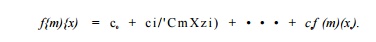
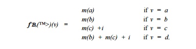
2.         If s is an assignment statement to variable x, then fs(m)(x)

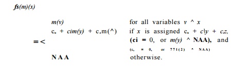
The expression CQ + cira(y) + c2m(z) is intended to represent all the possible forms of expressions involving arbitrary variables y and z that may appear on the right side of an assignment to x and that give x a value that is an affine transformation on prior values of variables. These expressions are: Co, Co + y, c o — Vi V + z i x — Vi c i * Vi a  n  d y / ( l / c i ) . Note that in many cases, one or more of Co, ci, and c 2 are 0.      

Example 9 . 6 0 :  If the assignment is x=y+z, then Co = 0 and c1 — c2   — 1.  If the assignment is x=y/5, then c0    = c2    = 0, and ci = 1/5.

Composition of Transfer Functions  

To compute f2 ° fi,  where  fi  and f2 are  defined in terms  of input  map  m, we substitute the value of m(vi)  in the  definition of f2    with the  definition of fi(m)(vi).  We replace all operations on NAA values with NAA.  That is,

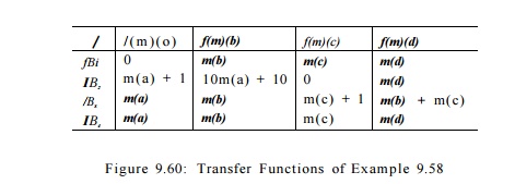
Example 9 . 6 1 : The transfer functions of the blocks in Example 9.58 can be computed by composing the transfer functions of their constituent statements. These transfer functions are defined in Fig. 9.60.

Solution  to  Data - Flow Problem 

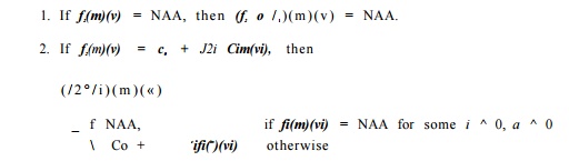
We  use the  notation  lNij[B3] and  OVTij[B3]  to  refer  to the  input and  output data-flow values of block B3 in iteration j of the inner loop and iteration i of the  outer  loop. For the other  blocks,  we  use  lNi[Bk] and  OUTi[Bk]  to  refer to these values in the ith iteration of the outer loop. Also,  we can see that

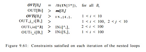
the symbolic maps shown in Fig. 9.58 satisfy the constraints imposed by the transfer functions, listed in Fig. 9.61.

The first constraint says that the output map of a basic block is obtained by applying the block's transfer function to the input map . The rest of the constraints say that the output map of a basic block must be greater than or equal to the input map of a successor block in the execution.

Note that our iterative data-flow algorithm cannot produce the above solu-tion because it lacks the concept of expressing data-flow values in terms of the number of iterations executed. Region-based analysis can be used to find such solutions, as we shall see in the next section.

3. Region-Based Symbolic Analysis

We can extend the region-based analysis described in Section 9.7 to find ex-pressions of variables in the ith. iteration of a loop. A region-based symbolic analysis has a bottom-up pass and a top-down pass, like other region-based al-gorithms. The bottom-up pass summarizes the effect of a region with a transfer function that sends a symbolic map at the entry to an output symbolic map at the exit. In the top-down pass, values of symbolic maps are propagated down to the inner regions.

The difference lies in how we handle loops.  In Section 9.7, the effect of a loop is summarized with a closure operator.  Given a loop with body /, its closure /* is defined as an infinite meet of all possible numbers of applications of /. However, to find induction variables, we need to determine if a value of a variable is an affine function of the number of iterations executed so far. The symbolic map must be parameterized by the number of the iteration being executed. Furthermore, whenever we know the total number of iterations executed in a loop, we can use that number to find the values of induction variables after the loop. For instance, in Example 9.58, we claimed that a has the value of i after executing the ith iteration. Since the loop has 100 iterations, the value of a must be 100 at the end of the loop.

In what follows, we first define the primitive operators:  meet and composition of transfer functions for symbolic analysis.  Then show how we use them to perform region-based analysis of induction variables.

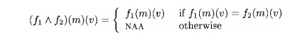
Meet  of Transfer  Functions

When computing the meet of two functions, the value of a variable is NAA unless the two functions map the variable to the same value and the value is not NAA. Thus,

Parameterized  Function  Compositions

To express a variable as an affine function of a loop index, we need to compute the effect of composing a function some given number of times. If the effect of one iteration is summarized by transfer function /, then the effect of executing i iterations, for some i > 0, is denoted /1 Note that when i = 0, fl = f° = I, the identify function.     

 Variables in the program are divided into three categories:    

1. If f(m)(x) = m(x)  + c,  where  c is  a constant,  then  fl(m)(x) — m(x) + ci  for every value of i > 0.  We say that a: is a basic induction variable of the loop whose body is represented by the transfer function /.   

2. If f(m)(x) =  m(x),  then  fl(m)(x)  =  m(x)  for  all  i  >  0. The  variable x is not modified and it remains unchanged at the end of any number of  iterations through the loop with transfer function /.  We say that x is a   symbolic  constant in  the  loop.     

3. l£f(m)(x) = co+cim(xi)-1 1-cnm(xn), where each xk is either a basic induction variable or a symbolic constant, then for i > 0,

We say that x is also an induction variable, though not a basic one. Note that the formula above does not apply if i = 0.

4.  In all other cases,  fl(m)(x)  = NAA.

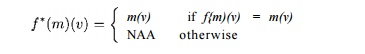
To find the effect of executing a fixed number of iterations, we simply replace i above by that number.  In the case where the number of iterations is unknown, the value at the start of the last iteration is given by /* .  In this case, the only variables whose values can still be expressed in the affine form are the loop-invariant variables.  

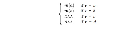
Example 9.62 :  For the innermost loop in Example 9.58, the effect of executing i iterations, i > 0, is summarized by / j ^ . From the definition of fBs, we see that a and 6 are symbolic constants, c is a basic induction variable as it is incremented by one every iteration, d is an induction variable because it is an affine function the symbolic constant b and basic induction variable c. Thus,

If we could not tell how many times the loop of block B3 iterated, then we could not use /* and would have to use /* to express the conditions at the end of the loop. In this case, we would have

A  Region - Based  Algorithm

Algorithm 9 . 63 :  Region-based symbolic analysis.

INPUT : A reducible flow graph G.

OUTPUT : Symbolic maps IN[B] for each block B of G.

METHOD : We make the following modifications to Algorithm 9.53.

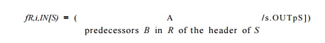
1. We change how we construct the transfer function for a loop region. In the original algorithm we use the /#,IN[.S] transfer function to map the symbolic map at the entry of loop region R to a symbolic map at the  entry of loop body S after executing an unknown number of iterations. It is defined to be the closure of the transfer function representing all paths leading back to the entry of the loop, as shown in Fig. 9.50(b). Here we define /jy,iN[S] t° represent the effect of execution from the start of the loop region to the entry of the ith. iteration. Thus,

2.       If the number of iterations of a region is known, the summary of the region       is computed by replacing i with the actual count.

3.       In the top-down pass, we compute   /jjt<)iN[B] to     find     the   symbolic map           associated with the entry of the ith   iteration of a loop.

4. In the case where the input value of a variable m(v) is used on the right-hand-side of a symbolic map in region R, and m(v) = NAA upon entry to thexregion, we introduce a new reference variable t, add assignment t = v to the beginning of region R, and all references of m(v) are replaced by t. If we did not introduce a reference variable at this point, the NAA value held by v would penetrate into inner loops.

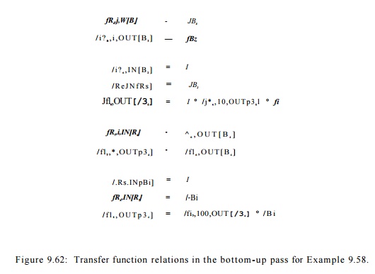
E x a m p l e 9 . 6 4 : For Example 9.58, we show how the transfer functions for the program are computed in the bottom-up pass in Fig. 9.62. Region R5 is the inner loop, with body B§. The transfer function representing the path from the entry of region R§ to the beginning of the j t h iteration, j > 1, is fB~X- The transfer function representing the path to the end of the j t h iteration, j > 1, is 4-

Region RQ consists of blocks B2 and B4, with loop region R$ in the middle. The transfer functions from the entry of B2 and R§ can be computed in the same way as in the original algorithm. Transfer function / R 6 , O U T [ B 3 ] represents the composition of block B2 and the entire execution of the inner loop, since fs4 is the identity function. Since the inner loop is known to iterate 10 times, we can replace j by 10 to summarize the effect of the inner loop precisely. The

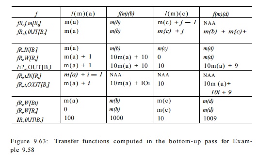
rest of the transfer functions can be computed in a similar manner. The actual transfer functions computed are shown in Fig. 9.63.

The symbolic map at the entry of the program is simply m N A A . We use the top-down pass to compute the symbolic map to the entry to successively nested regions until we find all the symbolic maps for every basic block. We start by

computing the data-flow values for block B1  in region Rs:

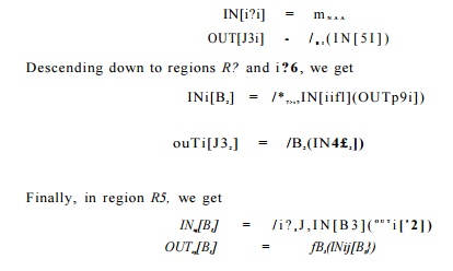
Not surprisingly, these equations produce the results we showed in Fig. 9.58.

Example 9.58 shows a simple program where every variable used in the symbolic map has an affine expression. We use Example 9.65 to illustrate why and how we introduce reference variables in Algorithm 9.63.

Example 9 . 6 5 : Consider the simple example in Fig. 9.64(a). Let fj be the transfer function summarizing the effect of executing j iterations of the inner loop. Even though the value of a may fluctuate during the execution of the loop, we see that b is an induction variable based on the value of a on entry of the  loop; that is, fj(m)(b)  — m(a) — 1+ j.  Because a is assigned an input value, the  symbolic map upon entry to the inner loop maps a to NAA.  We introduce a new reference  variable  t to save the value of a upon entry, and perform the substitutions as  in Fig.  9.64(b).

4. Exercises for Section 9.8

Exercise 9 . 8 . 1 :  For the flow graph of Fig. 9.10 (see the exercises for Section

9.1), give the transfer functions for

a)                 Block  B2.

b)          Block  B4.

c)           Block B5.

Exercise  9 . 8 . 2 :  Consider  the  inner loop of Fig. 9.10, consisting of blocks B3 and  B4.   If i  represents the  number  of times  around the  loop,  and / is the transfer function  for  the  loop  body  (i.e.,  excluding the  edge from  B4  to  B3) from the entry of the loop  (i.e., the  beginning of B3) to the exit from B4,  then what is /*? Remember that / takes as argument a map m, and m assigns a value to each of variables a, b, d, and e. We denote these values m(o), and so on, although we do not know their values.

Exercise 9 . 8 . 3 :  Now consider the outer  loop of Fig.  9.10, consisting of blocks B2,  B3,  B4,  and B5.    Let  g be the  transfer  function for  the loop body, from the entry of the loop  at  B2  to its exit  at B5.  Let i measure the number of iterations of the inner loop of  B3  and B4    (which count of iterations we cannot know), and let j measure the number of iterations of the outer loop (which we also cannot know). What is <?J?

Summary of Chapter 9

4- Global Common Subexpressions: An important optimization is finding computations of the same expression in two different basic blocks. If one precedes the other, we can store the result the first time it is computed and use the stored result on subsequent occurrences.

•                     Copy Propagation: A copy statement, u — v, assigns one variable v to another, u. In some circumstances, we can replace all uses of u by v, thus eliminating both the assignment and u.

•                     Code Motion: Another optimization is to move a computation outside the loop in which it appears. This change is only correct if the computation produces the same value each time around the loop.

•                     Induction Variables: Many loops have induction variables, variables that take on a linear sequence of values each time around the loop. Some of these are used only to count iterations, and they often can be eliminated,

thus reducing the time it takes to go around the loop.

• Data-Flow Analysis: A data-flow analysis schema defines a value at each point in the program. Statements of the program have associated transfer functions that relate the value before the statement to the value after. Statements with more than one predecessor must have their value defined by combining the values at the predecessors, using a meet (or confluence) operator.

block, respectively. The transfer functions for the statements in a block are composed to get the transfer function for the block as a whole.

4  Reaching  Definitions:  The  reaching-definitions  data-flow  framework  has values that are sets of statements in the program that define values for one or more  variables.  The transfer  function  for a block kills definitions of variables  that are  definitely redefined in the block and adds  ("generates" ) in those definitions of variables that occur within the block.  The   confluence operator is union, since definitions reach a point if they reach   any predecessor of that point.      

4  Live  Variables:  Another  important  data-flow  framework  computes  the   variables that  are live  (will  be  used before  redefinition)  at  each point.   The framework is similar to reaching definitions, except that the transfer   function runs backward.  A variable is live at  the beginning of a block if   it is either used before definition in the block or is live at the end of the   block and not redefined in the block.    

4  Available  Expressions:  To  discover  global  common  subexpressions,  we   determine the available expressions at each point — expressions that have   been computed and neither of the expression's arguments were redefined   after the last computation.  The data-flow framework is similar to reaching   definitions, but the confluence operator is  intersection rather than union.

4  Abstraction  of  Data-Flow  Problems:  Common  data-flow  problems,  such   as those already mentioned, can be expressed in a common mathematical   structure.  The values are members of a semilattice, whose meet is the   confluence operator.  Transfer functions  map lattice elements to lattice   elements.   The  set  of allowed transfer functions  must  be  closed  under   composition and include the identity function.

4  Monotone  Frameworks:  A  semilattice  has  a <  relation defined by a  <  b   if and only if a A b = a.  Monotone frameworks have the property that   each transfer function preserves the < relationship; that is, a < b implies   f{o)  < f(b), for all lattice  elements a and b and transfer function /.

4  Distributive  Frameworks:  These  frameworks  satisfy  the  condition  that   f{a/1b)  =  f(a)Af(b), for  all  lattice elements  a and b and transfer function   /.  It can be shown that the distributive condition implies the monotone    condition.             

4  Rerative  Solution  to  Abstract Frameworks:  All  monotone data-flow frame-   works  can  be  solved  by  an  iterative  algorithm,  in  which  the  IN  and   OUT  values  for  each  block  are  initialized  appropriately  (depending on   the framework), and new values for these variables are repeatedly computed by applying the transfer and confluence operations.  This solution is always  safe  (optimizations that it  suggests will not  change what the program does), but the solution is certain to be the best possible only if the framework is distributive.

• The Constant Propagation Framework: While the basic frameworks such as reaching definitions are distributive, there are interesting monotone-but-not-distributive frameworks as well. One involves propagating con-stants by using a semilattice whose elements are mappings from the pro-gram variables to constants, plus two special values that represent "no information" and "definitely not a constant."

• Partial-Redundancy Elimination: Many useful optimizations, such as code motion and global common-subexpression elimination, can be generalized to a single problem called partial-redundancy elimination. Expressions that are needed, but are available along only some of the paths to a point, are computed only along the paths where they are not available. The correct application of this idea requires the solution to a sequence of four different data-flow problems plus other operations.

• Dominators: A node in a flow graph dominates another if every path to the latter must go through the former. A proper dominator is a dominator other than the node itself. Each node except the entry node has an imme-diate dominator — that one of its proper dominators that is dominated by all the other proper dominators.

4  Depth-First  Ordering  of Flow  Graphs:  If we  perform  a depth-first  search   of a flow graph, starting at its entry, we produce a depth-first spanning   tree.   The depth-first  order of the nodes is the reverse of a postorder   traversal of this tree.      

4-  Classification  of Edges:  When we construct  a depth-first  spanning tree,   all the edges of the flow graph can be divided into three groups:  advancing edges (those that go from ancestor to proper descendant), retreating   edges (those from descendant to ancestor) and cross edges (others).  An   important property is that all the cross edges go from right to left in the   tree.  Another important property is that of these edges, only the retreating edges have a head lower than its tail in the depth-first order (reverse   postorder).       

•  Back Edges:  A back edge is  one whose head dominates its tail.  Every   back edge is a retreating edge, regardless of which depth-first spanning   tree for its flow graph is  chosen. 

4  Reducible Flow Graphs: If every retreating edge is a back edge, regardless of which depth-first spanning tree is chosen, then the flow graph is said to be reducible. The vast majority of flow graphs are reducible; those whose only control-flow statements are the usual loop-forming and branching statements are certainly reducible.

4                   Natural Loops: A natural loop is a set of nodes with a header node that dominates all the nodes in the set and has at least one back edge entering that node. Given any back edge, we can construct its natural loop by taking the head of the edge plus all nodes that can reach the tail of the edge without going through the head. Two natural loops with different headers are either disjoint or one is completely contained in the other; this fact lets us talk about a hierarchy of nested loops, as long as "loops" are taken to be natural loops.

4 Depth-First Order Makes the Rerative Algorithm Efficient: The iterative algorithm requires few passes, as long as propagation of information along acyclic paths is sufficient; i.e., cycles add nothing. If we visit nodes in depth-first order, any data-flow framework that propagates information forward, e.g., reaching definitions, will converge in no more than 2 plus the largest number of retreating edges on any acyclic path. The same holds for backward-propagating frameworks, like live variables, if we visit in the reverse of depth-first order (i.e., in postorder).

4 Regions: Regions are sets of nodes and edges with a header h that domi-nates all nodes in the region. The predecessors of any node other than h in the region must also be in the region. The edges of the region are all

that go between nodes of the region, with the possible exception of some

or all that enter the header.

4                   Regions and Reducible Flow Graphs: Reducible flow graphs can be parsed into a hierarchy of regions. These regions are either loop regions, which include all the edges into the header, or body regions that have no edges into the header.

Region-Based  Data-Flow  Analysis:  An  alternative  to  the  iterative  approach to data-flow analysis is to work up and down the region hierarchy, computing transfer functions from the header of each region to each node in that region.   

Region-Based  Induction  Variable  Detection:  An  important  application  of region-based analysis is in a data-flow framework that tries to compute formulas for each variable in a loop region whose value is an affine (linear) function of the number  of times  around the loop.