State space representation of Continuous Time systems

State space representation of Continuous Time systems

The state variables may be totally independent of each other, leading to diagonal or normal form or they could be derived as the derivatives of the output. If them is no direct relationship between various states. We could use a suitable transformation to obtain the representation in diagonal form.

Phase Variable Representation

It is often convenient to consider the output of the system as one of the state variable and remaining state variable as derivatives of this state variable. The state variables thus obtained from one of the system variables and its (n-1) derivatives, are known as n-dimensional phase variables.

In a third-order mechanical system, the output may be displacement x1, x1= x2= v and x2 = x3 = a in the case of motion of translation or angular displacement θ 1 = x1, x1= x2= w and x2 = x3 = α if the motion is rotational, Where v v,w,a, α respectively, are velocity, angular velocity acceleration, angular acceleration.

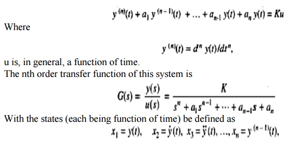
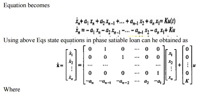
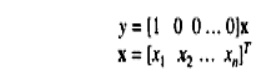
Consider a SISO system described by nth-order differential equation.

Physical Variable Representation

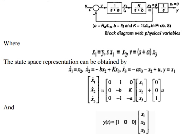
In this representation the state variables are real physical variables, which can be measured and used for manipulation or for control purposes. The approach generally adopted is to break the block diagram of the transfer function into subsystems in such a way that the physical variables can he identified. The governing equations for the subsystems can he used to identify the physical variables. To illustrate the approach consider the block diagram of Fig.

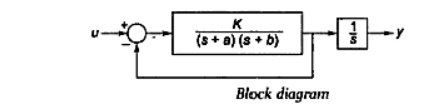
One may represent the transfer function of this system as

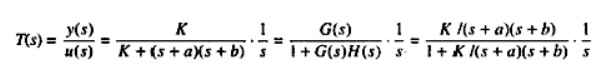
Taking H(s) = 1, the block diagram of can be redrawn as in Fig. physical variables can be speculated as x1=y, output, x2 =w= θ the angular velocity x3 = Ia the armature current in a position-control system.