Selected LP Applications: Manpower Planning

SELECTED LP APPLICATIONS

This section presents realistic LP models in which the definition of the variables and the construction of the objective function and constraints are not as straight-forward as in the case of the two-variable model. The areas covered by these appli-cations include the following:

1. Urban planning.

2. Currency arbitrage.

3. Investment.

4. Production planning and inventory control.

5. Blending and oil refining.

6. Manpower planning.

Each model is fully developed and its optimum solution is analyzed and interpreted.

6. Manpower Planning

Fluctuations in a labor force to meet variable demand over time can be achieved through the process of hiring and firing, as demonstrated in Example 2.3-6. There are situations in which the effect of fluctuations in demand can be "absorbed" by adjusting the start and end times of a work shift. For example, instead of following the tradition-al three 8-hour-shift start times at 8:00 A.M., 3:00 P.M., and 11:00 P.M., we can use over-lapping 8-hour shifts in which the start time of each is made in response to increase or decrease in demand.

The idea of redefining the start of a shift to accommodate fluctuation in demand can be extended to other operating environments as well. Example 2.3-8 deals with the determination of the minimum number of buses needed to meet rush-hour and off-hour transportation needs.

Real-Life Application-Telephone Sales Manpower Planning at Qantas Airways

Australian airline Qantas operates its main reservation offices from 7:00 till 22:00 using 6 shifts that start at different times of the day. Qantas used linear programming (with imbedded queuing analysis) to staff its main telephone sales reservation office efficiently while providing convenient service to its customers. The study, carried aut in the late 1970s, resulted in annual savings of over 200,000 Australian dollars per year. The study is detailed in Case 15, Chapter 24 on the CD.

Example 2.3-8        (Bus Scheduling)

Progress City is studying the feasibility of introducing a mass-transit bus system that will alleviate the smog problem by reducing in-city driving. The study seeks the minimum number of buses that can handle the transportation needs. After gathering necessary information, the city engi-neer noticed that the minimum number of buses needed fluctuated with the time of the day and that the required number of buses could be approximated by constant values over successive 4-hour intervals. Figure 2.8 summarizes the engineer's findings. To carry out the required daily maintenance, each bus can operate 8 successive hours a day only.

Mathematical Model: Determine the number of operating buses in each shift (variables) that will meet the minimum demand (constraints) while minimizing the total number of buses in op-eration (objective).

You may already have noticed that the definition of the variables is ambiguous. We know that each bus will run for 8 consecutive hours, but we do not know when a shift should start. If we follow a normal three-shift schedule (8:01 A.M.-4:00 P.M., 4:01 p.M.-12:00 midnight, and 12:01 A.M.-8:00 A.M.) and assume that  x₁,x₂ and x₃ are the number of buses starting in the first, second, and third shifts, we can see from Figure 2.8 that x_l ≥ 10, x2 ≥ 12, and X3 ≥ 8. The corre-sponding minimum number of daily buses is x₁ + x₂ + x₃ = 10 + 12 + 8 = 30.

The given solution is acceptable only if the shifts must coincide with the norma) three-shift schedule. It may be advantageous, however, to allow the optimization process to choose the "best" starting time for a shift. A reasonable way to accomplish this is to allow a shift to start every 4 hours. The bottom of Figure 2.8 illustrates this idea where overlapping 8-hour shifts

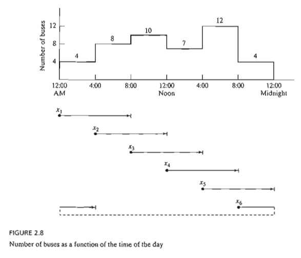
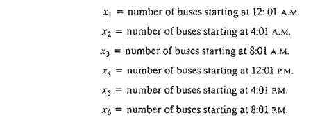
may start at 12:01 A.M., 4:01 A.M., 8:01 A.M., 12:01 P.M., 4:01 P.M., and 8:01 P.M. Thus, the variables may be defined as

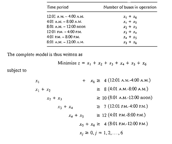
We can see from Figure 2.8 that because of the overlapping of the shifts, the number of buses for the successive 4-hour periods is given as

Solution:

The optimal solution calls for using 26 buses to satisfy the demand with x. = 4 buses to start at 12:01 A.M., x₂ = 10 at 4:01 A.M., x₄ = 8 at 12:01 P.M., and x₅ = 4 at 4:01 P.M.

PROBLEM SET 2.3F

*1. In the bus scheduling example suppose that buses can run either 8- or 12-hour shi-fts. If a bus runs for 12 hours, the driver must be paid for the extra hours at 150% of the regular hourly pay. Do you recommend the use of 12-hour shifts?

2. A hospital employs volunteers to staff the reception desk between 8:00 A.M. and 10:00 P.M. Each volunteer works three consecutive hours except for those starting at 8:00 P.M. who work for two hours only. The minimum need for volunteers is approximated by a step function over 2-hour intervals starting at 8:00 A.M. as 4, 6, 8, 6, 4, 6, 8. Because most volun-teers are retired individuals, they are willing to offer their services at any hour of the day (8:00 A.M. to 10:00 P.M.). However, because of the large number of charities competing for their service, the number needed must be kept as low as possible. Determine an optimal schedule for the start time of the volunteers

3. In Problem 2, suppose that no volunteers will start at noon or 6:00 P.M. to allow for lunch and dinner. Determine the optimal schedule.

4. In an LTL (less-than-truckload) trucking company, terminal docks include casual work-ers who are hired temporarily to account for peak loads. At the Omaha, Nebraska, dock, the minimum demand for casual workers during the seven days of the week (starting on Monday) is 20, 14, 10, 15, 18, 10, 12 workers. Each worker is contracted to work five con-secutive days. Determine an optimal weekly hiring practice of casual workers for the company.

*5. On most university campuses students are contracted by academic departments to do er-rands, such as answering the phone and typing. The need for such service fluctuates dur-ing work hours (8:00 A.M. to 5:00 P.M.). In the IE department, the minimum number of students needed is 2 between 8:00 A.M. and 10:00 A.M.,3 between 10:01 A.M. and 11:00 A.M.,4 between 11:01 A.M. and 1:00 P.M., and 3 between 1:01 P.M. and 5:00 P.M. Each stu-dent is allotted 3 consecutive hours (except for those starting at 3:01, who work for 2 hours and those who start at 4:01, who work for one hour). Because of their flexible schedule, students can usually report to work at any hour during the work day, except that no student wants to start working at lunch time (12:00 noon). Determine the mini-mum number of students the IE department should employ and specify the time of the day at which they should report to work.

6. A large department store operates 7 days a week. The manager estimates that the mini-mum number of salespersons required to provide prompt service is 12 for Monday, 18 for Tuesday, 20 for Wednesday, 28 for Thursday, 32 for Friday, and 40 for each of Saturday' and Sunday. Each salesperson works 5 days a week, with the two consecutive off-days staggered throughout the week. For example, if 10 salespersons start on Monday, two can take their off-days on Tuesday and Wednesday, five on Wednesday and Thursday, and three on Saturday and Sunday. How many salespersons should be contracted and how should their off-days be allocated?