Root Locus Technique, Analysis and Application Procedure

Root Locus Technique

o   Introduced by W. R. Evans in 1948

o   Graphical method, in which movement of poles in the s-plane is sketched when some parameter is varied The path taken by the roots of the characteristic equation when open loop gain K is varied from 0 to ∞ are called root loci

o   Direct Root Locus = 0 < k < ∞

o   Inverse Root Locus = - ∞ < k < 0

Root Locus Analysis:

o   The  roots  of  the  closed-loop  characteristic  equation  define  the  system  characteristic responses

o   Their location in the complex s-plane lead to prediction of the characteristics of the time domain responses in terms of:

o   damping ratio ζ,

o   natural frequency, wn

o   damping constant ζ, first-order modes

o   Consider how these roots change as the loop gain is varied from 0 to∞

Basics of Root Locus:

o   Symmetrical about real axis

o   RL branch starts from OL poles and terminates at OL zeroes

o   No. of RL branches = No. of poles of OLTF

o   Centroid is common intersection point of all the asymptotes on the real axis

o   Asymptotes are straight lines which are parallel to RL going to ∞ and meet the RL at ∞

o   No. of asymptotes = No. of branches going to ∞

o   At Break Away point , the RL breaks from real axis to enter into the complex plane

o   At BI point, the RL enters the real axis from the complex plane

Constructing Root Locus:

o   Locate the OL poles & zeros in the plot Find the branches on the real axis

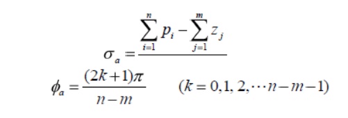
o   Find angle of asymptotes & centroid

o   Φa= ±180º(2q+1) / (n-m)

o   ζa = (Σpoles - Σzeroes) / (n-m) Find BA and BI points

o   Find Angle Of departure (AOD) and Angle Of Arrival (AOA)

o   AOD = 180º- (sum of angles of vectors to the complex pole from all other poles) + (Sum of angles of vectors to the complex pole from all zero)

o   AOA = 180º- (sum of angles of vectors to the complex zero from all other zeros) + (sum of angles of vectors to the complex zero from poles)

o   Find the point of intersection of RL with the imaginary axis.

Application of the Root Locus Procedure

Step 1: Write the characteristic equation as

1+ F(s)= 0

Step 2: Rewrite preceding equation into the form of poles and zeros as follows

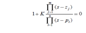
Step 3:

Locate the poles and zeros with specific symbols, the root locus begins at the open-loop poles and ends at the open loop zeros as K increases from 0 to infinity

If open-loop system has n-m zeros at infinity, there will be n-m branches of the root locus approaching the n-m zeros at infinity

Step 4:

The root locus on the real axis lies in a section of the real axis to the left of an odd number of real poles and zeros

Step 5:

The number of separate loci is equal to the number of open-loop poles

Step 6:

The root loci must be continuous and symmetrical with respect to the horizontal real axis

Step 7:

The loci proceed to zeros at infinity along asymptotes centered at centroid and with angles

Step 8:

The actual point at which the root locus crosses the imaginary axis is readily evaluated by using Routh‗s criterion

Step 9:

 Determine the breakaway point d (usually on the real axis)

Step 10:

Plot the root locus that satisfy the phase criterion

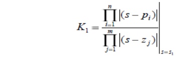
Step 11:

Determine the parameter value K1 at a specific root using the magnitude criterion