Chapter: Civil : Structural dynamics of earthquake engineering
Response of structures to periodic dynamic loadings
Response
of structures to periodic dynamic loadings
Abstract: In many real problems, it is
found that exciting forces vary with time in a non-harmonic fashion that
may be periodic or non-periodic. When the function defined over a period
repeats indefinitely, it is known as a periodic function. In this page, we
apply the Fourier series to determine the response of the system to periodic
forces.
Key words: periodic function, Fourier
series, odd function, even function, frequency domain, spectrum, Gibbs
phenomenon.
Introduction
We have seen in Chapter 4 that
harmonic excitation occurs in power installations equipped with rotating and
reciprocating machinery. The solution to harmonic excitation is simple and
straightforward since a closed form solution is always available. In many
realistic situations, the exciting forces vary with time in a non-harmonic
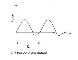
fashion that may be periodic or non-periodic. A periodic function is one in
which the portion defined over a period T0 repeats itself
indefinitely, (see Fig. 5.1). Propeller force on a ship, wind loading induced
by vortex shedding on tall slender structures are the examples of periodic
forces, whereas, earthquake ground motion has no resemblance to periodic
function.
This chapter presents the application of Fourier series to
determine the response of a system to periodic forces in the frequency domain,
an alternative approach to the usual analysis of time domain. To make practical
use of Fourier method, it is necessary to replace the integration with finite
sums.
Fourier analysis
Consider an undamped
single-degree-of-freedom (SDOF) system subjected to force F(t)
The governing equation is written as
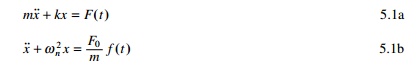
Let the forcing function be
represented as shown in Fig. 5.2. The duration of one pulse or period T0
= 4s.
F(t)
= 10 t <2 s
F(t)
= Ð10 2 < t < 4 5.2
Fourier has shown that a periodic function can be expressed as
a sum of infinite number of sine and cosine terms and such a sum is known as a
Fourier series.
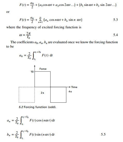
t1 in Eq.
5.5 can take any value of time, but is usually Ð T/2 or zero. Note that
Fourier coefficients a1, an, bn
may be expedited if the forcing function can be recognized as being odd or
even. If the forcing function is anti-symmetric about the origin (y-axis)
then it is an odd function. For example, the given function shown in Fig. 5.2
is an odd function because

For an odd function, the Fourier coefficients a0,
a1,├ē, an = 0
The forcing function is even if

For an even function, the Fourier coefficients b0,
b1,├ē, bn = 0
Clearly then an odd function can
be represented by the Fourier sine series and an even function by the Fourier
cosine series. If, however, the function is neither odd nor even, then the full
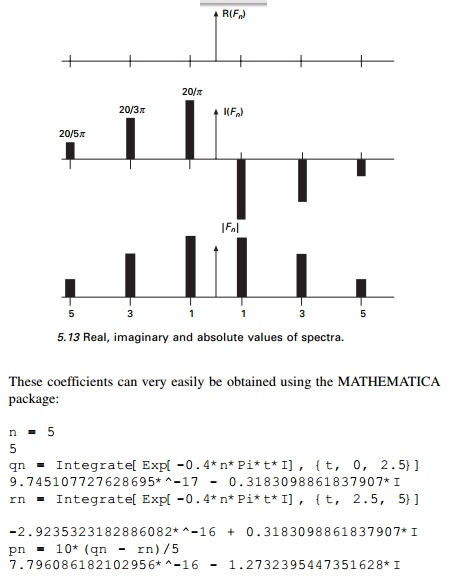
Fourier series must be employed. The Fourier coefficients can very easily be
evaluated using the MATHEMATICA package as shown by the following examples.
Example 5.1
Determine the Fourier series
expression for the square wave, periodic function as shown in Fig. 5.2. Plot
the Fourier representation for the first four non-zero harmonic components.
(Assume F0 = 10)
Solution
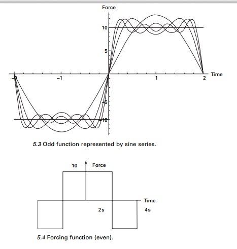
Since the forcing function is an odd function, the Fourier
coefficients a0, a1,├ē, an =
0. Thus the forcing function is represented by the Fourier sine series
as
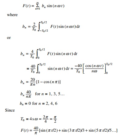
The forcing function is
represented in Fig. 5.3 in terms of 1, 2, 3 and 4 non-zero terms of Fourier
series.
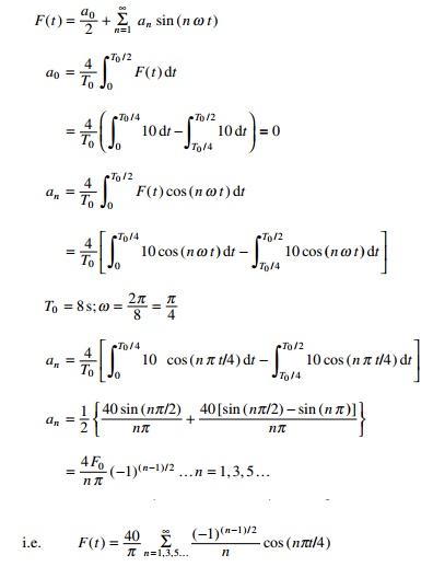
Example 5.2
Determine the Fourier series expression for square wave
periodic forcing function as shown in Fig. 5.4. Plot the Fourier representation
of the first four non-zero components.
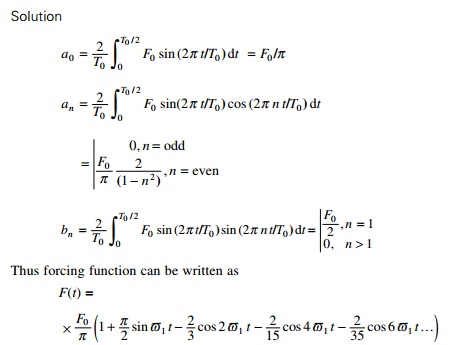
Solution
Since F(t) is an even function, b1,
b2, bn are zero. Thus ├'a├Ģ
coefficients are represented by Fourier cosine series as
In Fig. 5.5 the forcing function
is represented in terms of 1, 2, 3, 4 non-zero terms of cosine series.
The
MATHEMATICA program is used to find the Fourier coefficients.
Example 5.3
Determine the Fourier series expansion for a square wave
periodic forcing function as shown in Fig. 5.6. Plot the Fourier representation
of the first four non-zero components
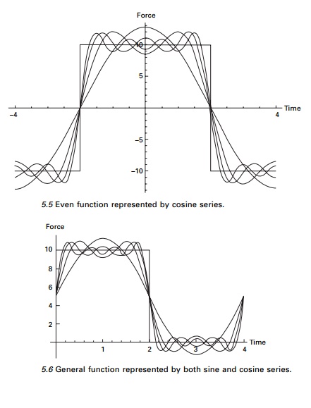
Solution
Since F(t) is
neither odd nor even function, this should contain both sine and cosine terms.
In Fig. 5.6 the forcing function is represented in terms of 1, 2, 3 and 4
non-zero terms of Fourier series.
Response to periodic
excitation
Next, consider the response of a viscously damped SDOF system
to periodic non-harmonic excitation of period T0. The
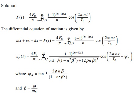
differential equation of motion of steady state response is given by
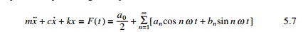
in which Fourier series expansion was used to represent F(t).
The transient response will decay with time and is hence neglected. To obtain
the particular solution for the steady state response, it is noted that
differential equation is linear, and therefore principle of superposition is
applicable. Hence the steady state response is merely the sum of the individual
particular solutions for all harmonic terms representing F(t).
Hence we obtain
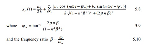
in which Žłn is the
phase angle for the steady state response.
Example 5.4
For the harmonic periodic forcing function shown in Fig. 5.5
determine the steady state response for a viscously under-damped SDOF system.
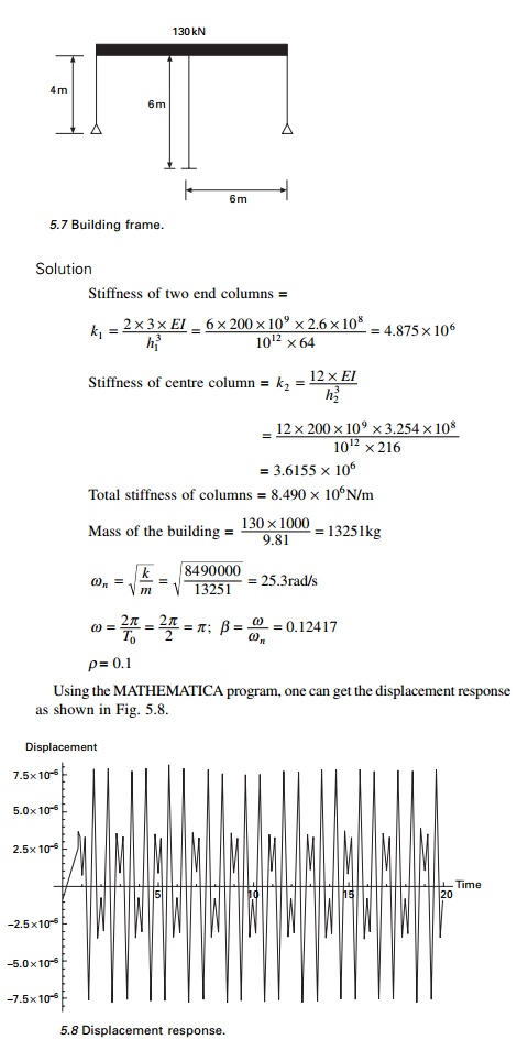
Example 5.5
The building frame shown in Fig. 5.7 is constructed of rigid
girders and flexible columns. The frame supports a uniformly distributed load
of weight of 130kN and is subjected at its girder level to the periodic force
described in Fig. 5.4. Evaluate the steady state response of the structure and
plot displacement vs. time assuming F0 = 80kN, period of
exciting force is 2 s, E = 200GPa, damping factor = 0.1, height of end
columns is 4m, the height of centre column is 6m and the span of the beams is
6m. The values of I for end columns and centre column are 2.6 ├- 108 and 3.254 ├- 108mm4
respectively.
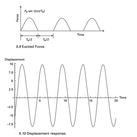
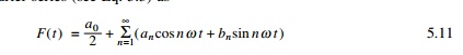
Example 5.6
Consider a system loaded as shown in Fig. 5.9. Find the steady
state response.
in which Ž- = 2ŽĆ/T0.
Using the MATHEMATICA program, the displacement response is
obtained for ╬▓ = ŽĆ/4, T0 = 4s Žü = 0.25 as shown in Fig. 5.10.
Frequency domain analysis
The dynamic response of the complex systems can be examined by
two approaches: time domain solution and the frequency domain solution. Up to
now, all solutions have been in time domain and the equations are solved by
integrating with time. In
frequency domain technique, the amplitude coefficients in the Fourier series
solution corresponding to each frequency are determined. For this we use
discrete Fourier transform (DFT) or fast Fourier transform (FFT) methods.
Alternative form of
Fourier series
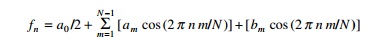
The arbitrary periodic forcing function can be represented in
the form of Fourier series (see Eq. 5.3) as
in which a0, a1├ē
an, b1, b2, ├ē bn
are real constants, t is the time and Žē is the forcing frequency given by Žē = 2ŽĆ/T0 where T0
is the period of the forcing function. If the period of the forcing function is
not known or if the forcing function does not have period for this case Žē = 2ŽĆ/TD where TD
is the total time duration of the forcing function.
Equation 5.11 may also be written as
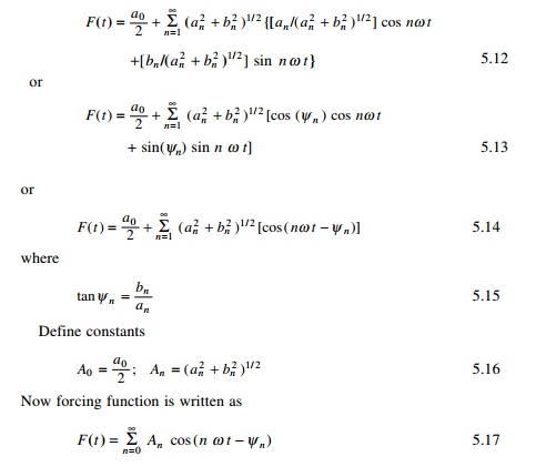
in which Žł0 = 0.
Hence forcing function is now written in terms of positive real amplitude and
phase shift. This method replaces the coefficients of an, bn
by An, Žłn. There is still the same number
of coefficients. The plots of An and Žłn are
called amplitude spectrum and phase spectrum respectively. They are discrete
and occur at Fourier frequencies nŽē = (2ŽĆ n)/TD.
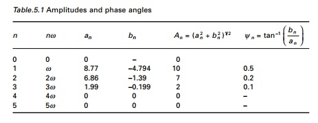
Example 5.7
A periodic load function of three frequency components is
given by
F(t) = 10 cos (Žē t - 0.5) +
7 cos (2Žē t - 0.2) +
2 cos (3 Žē t - 0.1)
in which Žē = 2ŽĆ/TD and TD
= 5s. Plot the periodic function and the amplitude and phase spectrum.
Solution
The equation for the coefficients are given as
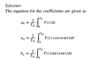
except that we use TD as fundamental period.
Evaluating the integrals in the above equations yields the values given in
Table 5.1.
Program 5.3: MATLAB
program to evaluate amplitudes and phase angles
clc; close all;
for i=1:200 t(i)=(i-1)/40;
p(i)=10*cos(2*pi*t(i)/5Ð0.5)+7.0*cos(4*pi*t(i)/5Ð0.2)+2.0*cos(6.0*pi*t(i)/
5Ð0.1) end figure(1) plot(t,p)
xlabel(' t');
ylabel('p(t)');
title(' time series plot');
figure(2)
a=fft(p);
plot(abs(a)); title(' amplitude')
for i=1:200
b(i)=real(a(i));
c(i)=imag(a(i)); d(i)=atan(-c(i)/b(i));
e(i)=sqrt(b(i)^2+c(i)^2);
end
print{' real part',\n); b
print(' imaginary part',\n); c
print(' phase angle',\n); d
print(' amplitude',\n)' e
figure(3)
plot(d); title(' phase')
figure(4);
plot(t,b,t,c,'*');
title(' real and imaginary part(*)')
The forcing function F(t) examined in Example
5.6 is rather a simple function, although, from the plot presented in Fig.
5.11a it is not readily
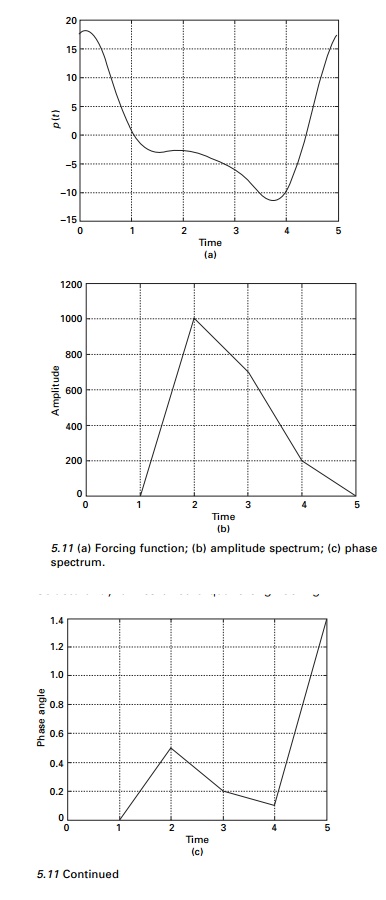
apparent that this is a simple
function. However the amplitude and phase spectrum parts shown in Fig. 5.11b
and 5.11c reveal clearly three cosines and their phases. As functions become
more complex with many frequency components, plots of amplitude spectra become
even more important in understanding the structure of the functions.
Example 5.8
A simple periodic load is characterized by the following
deterministic amplitude coefficients
Expression of forcing
function using complex variable approach
The forcing function is written as
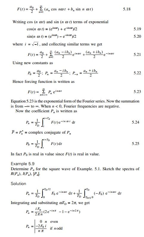
The exponential form is more convenient to use than the real
form. To illustrate the fact, consider SDOF system subjected to harmonic
forcing. The equation of motion is given by
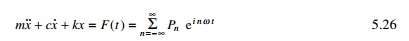
The steady state solution of Eq. 5.26 will respond to same
frequencies making up the forcing function.
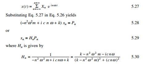
Writing in this way, the response at each frequency is simply
a function of the forcing transfer function. For a given structure H
depends only on frequency nŽē. This is termed the frequency domain solution. Consider ╬▓ as the
frequency ratio and Žü as the
damping factor. The function Hn is written as
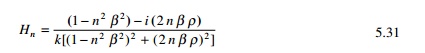
The phase is now defined as
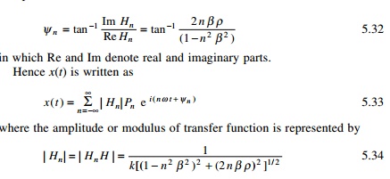
where Hn* is the complex
conjugate of Pn and Žån is the phase. It is to be noted
that forcing function Pn can be complex. Expressing Pn
as a modulus and phase we get

Since the spectral coefficients are even, this implies that a
spectrum plot we can consider either all frequencies between ├ÉŌł× and Ōł×
or just frequencies from 0 to Ōł× and
double the heights. The former is called a double-sided spectrum and the latter
is called a single-sided spectrum. Both spectra are reasonable representations
and both are used in practice.
Discrete Fourier
transform (DFT) and fast Fourier transform (FFT)
Although Fourier integral
technique discussed in previous sections provide a means for determining the
transient response of a system, numerical integral of the Fourier integral
became a practical reality only with the publication of Cooley-Tukey algorithm
for the FFT in 1965. Since that date, FFT has revolutionized many areas of
technology such as the areas of measurements and instrumentation.
Two steps are involved in the numerical evaluation of Fourier
transforms. DFTs correspond to the equation
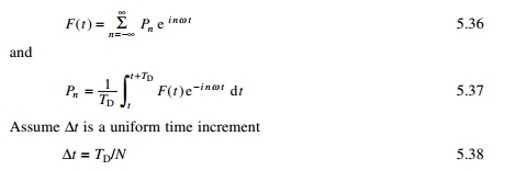
where N is the number of points in the time series
approximation of F(t). We can write
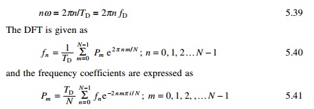
The total number of discrete time values and
frequency values are same. The N term appearing before the summation in
Eq. 5.40 is not unique. In
Root o
DFT it can be used as 1/N in Eqs. 5.40 and 5.41 or N
Root in both.
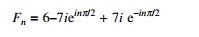
Example 5.10
Determine the DFT of the following function defined by
f (n Ōłåt) = 6 +
14 sin (nŽĆ/2) ├ē
n = 0, 1, 2,├ē, 7
Solution
In this example N = 8 and all coefficients are zero
except a0 = 12; b2 = 14. For this problem
the solution could be determined by inspection. With use of the Euler formulae,
the time series is written as
The transform of the series is given by
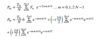
These coefficients may be evaluated using the MATHEMATICA package
and given by
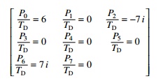
These are the same coefficients
that were determined by inspection of equation defining Pn, Pm
= Pm+n or PÐ2 = P6.
Gibbs phenomenon
The Fourier series approximation of a square wave has been
plotted in Fig. 5.34. The approximation is generally quite good as shown in the
figure. However, an inaccuracy exists at the corners of the wave. Sines and
cosines are smooth, continuous functions and therefore are best suited to
approximately other smooth and continuous functions. However, jumps or
discontinuities exist in them and the approximation is poor. For the square
wave a discontinuity exists at t/T0 = 0.5. At this
location, the square wave has two values +1 and Ð1. When the function has jumps
or double values, a Fourier series passes through the mean of the two points as
shown in Fig. 5.34, which in our case is zero. It is also to be noted that t/T0
= 0.5 the square wave is vertical. The fourier series tends to overshoot at the
corners. This is called the Gibbs phenomenon. This does not
disappear even if large number of terms are used
in the series. It is concluded that the Gibbs phenomenon is
local and the contribution to total energy is minimal.
Summary
Fourier integrals can be evaluated numerically. There are a
number of software packages available to do this, such as MATHEMATICA and
MATLAB. DFT has a finite number of frequencies and Fourier integrals have
continuous frequencies in the interval ├ÉŌł×
< f < Ōł× and high
frequency terms are lost. The other way of doing the Fourier integral is to use
polynomial interpolation functions which can be integrated analytically over
most of the data.
Related Topics