Propagation of Uncertainty

Propagation of Uncertainty

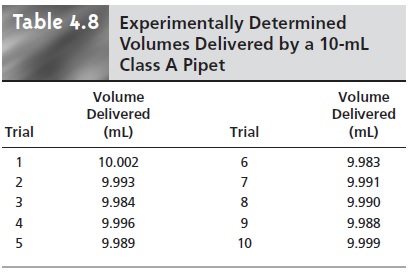
Suppose that you need to add a reagent to a flask by several successive transfers using a class A 10-mL pipet. By calibrating the pipet (see Table 4.8), you know that it delivers a volume of 9.992 mL with a standard deviation of 0.006 mL. Since the pipet is calibrated, we can use the standard deviation as a measure of uncertainty. This uncertainty tells us that when we use the pipet to repetitively deliver 10 mL of solution, the volumes actually delivered are randomly scattered around the mean of 9.992 mL.

If the uncertainty in using the pipet once is 9.992 ± 0.006 mL, what is the un- certainty when the pipet is used twice? As a first guess, we might simply add the un- certainties for each delivery; thus

(9.992 mL + 9.992 mL) ± (0.006 mL + 0.006 mL) = 19.984 ± 0.012 mL

It is easy to see that combining uncertainties in this way overestimates the total un- certainty. Adding the uncertainty for the first delivery to that of the second delivery assumes that both volumes are either greater than 9.992 mL or less than 9.992 mL. At the other extreme, we might assume that the two deliveries will always be on op- posite sides of the pipet’s mean volume. In this case we subtract the uncertainties for the two deliveries,

(9.992 mL + 9.992 mL) ± (0.006 mL – 0.006 mL) = 19.984 ± 0.000 mL

underestimating the total uncertainty.

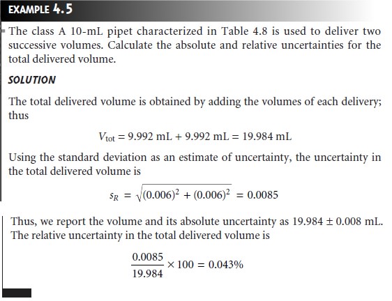
So what is the total uncertainty when using this pipet to deliver two successive volumes of solution? From the previous discussion we know that the total uncer- tainty is greater than ±0.000 mL and less than ±0.012 mL. To estimate the cumula- tive effect of multiple uncertainties, we use a mathematical technique known as the propagation of uncertainty. Our treatment of the propagation of uncertainty is based on a few simple rules that we will not derive. A more thorough treatment can be found elsewhere.

A Few Symbols

Propagation of uncertainty allows us to estimate the uncertainty in a calculated re- sult from the uncertainties of the measurements used to calculate the result. In the equations presented in this section the result is represented by the symbol R and the measurements by the symbols A, B, and C. The corresponding uncertainties are s_R, s_A, s_B, and s_C. The uncertainties for A, B, and C can be reported in several ways, in- cluding calculated standard deviations or estimated ranges, as long as the same form is used for all measurements.

Uncertainty When Adding or Subtracting

When measurements are added or subtracted, the absolute uncertainty in the result is the square root of the sum of the squares of the absolute uncertainties for the in- dividual measurements. Thus, for the equations R = A + B + C or R = A + B – C, or any other combination of adding and subtracting A, B, and C, the absolute uncer- tainty in R is

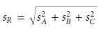                          4.6

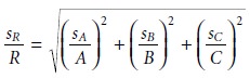
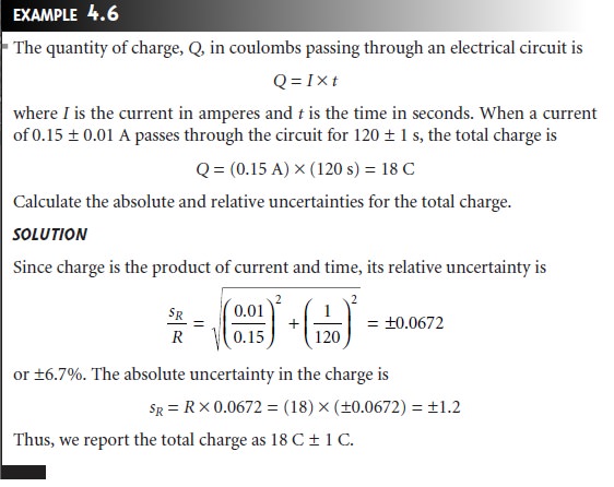
Uncertainty When Multiplying or Dividing

When measurements are multiplied or divided, the relative uncertainty in the result is the square root of the sum of the squares of the relative uncertainties for the indi- vidual measurements. Thus, for the equations R = A x B x C or R = A x B/C, or any other combination of multiplying and dividing A, B, and C, the relative uncertainty in R is

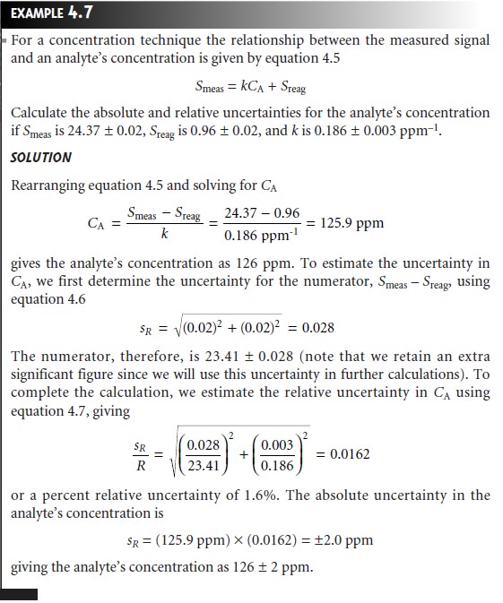
Uncertainty for Mixed Operations

Many chemical calculations involve a combination of adding and subtracting, and multiply and dividing. As shown in the following example, the propagation of un- certainty is easily calculated by treating each operation separately using equations 4.6 and 4.7 as needed.

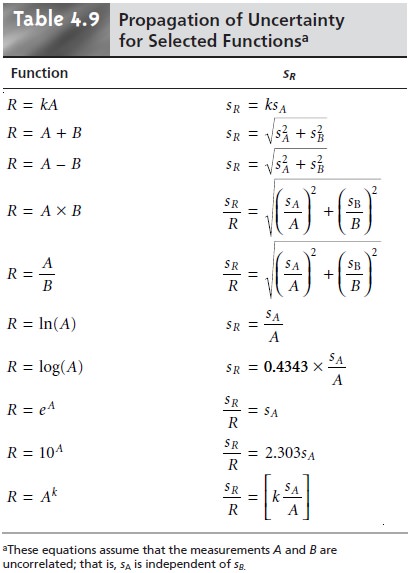
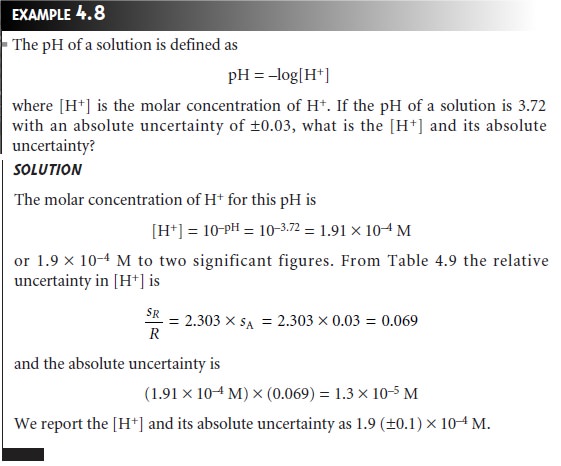
Uncertainty for Other Mathematical Functions

Many other mathematical operations are commonly used in analytical chemistry, including powers, roots, and logarithms. Equations for the propagation of uncer- tainty for some of these functions are shown in Table 4.9.

Is Calculating Uncertainty Actually Useful?

Given the complexity of determining a result’s uncertainty when several mea- surements are involved, it is worth examining some of the reasons why such cal- culations are useful. A propagation of uncertainty allows us to estimate an ex- pected uncertainty for an analysis. Comparing the expected uncertainty to that which is actually obtained can provide useful information. For example, in de- termining the mass of a penny, we estimated the uncertainty in measuring mass as ±0.002 g based on the balance’s tolerance. If we measure a single penny’s mass several times and obtain a standard deviation of ±0.020 g, we would have reason to believe that our measurement process is out of control. We would then try to identify and correct the problem.

A propagation of uncertainty also helps in deciding how to improve the un- certainty in an analysis. In Example 4.7, for instance, we calculated the concen- tration of an analyte, obtaining a value of 126 ppm with an absolute uncertainty of ±2 ppm and a relative uncertainty of 1.6%. How might we improve the analy- sis so that the absolute uncertainty is only ±1 ppm (a relative uncertainty of 0.8%)? Looking back on the calculation, we find that the relative uncertainty is determined by the relative uncertainty in the measured signal (corrected for the reagent blank)

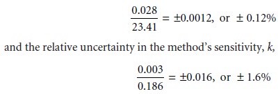
Of these two terms, the sensitivity’s uncertainty dominates the total uncertainty. Measuring the signal more carefully will not improve the overall uncertainty of the analysis. On the other hand, the desired improvement in uncertainty can be achieved if the sensitivity’s absolute uncertainty can be decreased to ±0.0015 ppm–1.

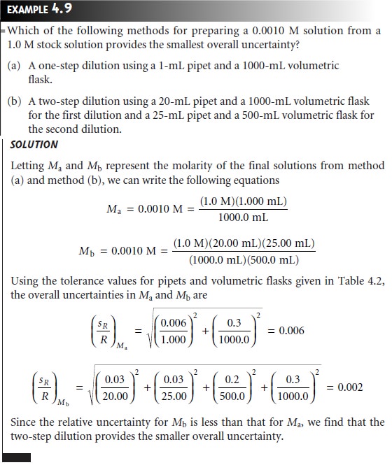
As a final example, a propagation of uncertainty can be used to decide which of several procedures provides the smallest overall uncertainty. Preparing a solu- tion by diluting a stock solution can be done using several different combina- tions of volumetric glassware. For instance, we can dilute a solution by a factor of 10 using a 10-mL pipet and a 100-mL volumetric flask, or by using a 25-mL pipet and a 250-mL volumetric flask. The same dilution also can be accom- plished in two steps using a 50-mL pipet and a 100-mL volumetric flask for the first dilution, and a 10-mL pipet and a 50-mL volumetric flask for the second di- lution. The overall uncertainty, of course, depends on the uncertainty of the glassware used in the dilutions. As shown in the following example, we can use the tolerance values for volumetric glassware to determine the optimum dilution strategy.