Overview of Titrimetry

Overview of Titrimetry

Titrimetric methods are classified into four groups based on the type of reaction in- volved. These groups are acid–base titrations, in which an acidic or basic titrant re- acts with an analyte that is a base or an acid; complexometric titrations involving a metal–ligand complexation reaction; redox titrations, where the titrant is an oxidiz- ing or reducing agent; and precipitation titrations, in which the analyte and titrant react to form a precipitate. Despite the difference in chemistry, all titrations share several common features, providing the focus for this section.

Equivalence Points and End Points

For a titration to be accurate we must add a stoichiometrically equivalent amount of titrant to a solution containing the analyte. We call this stoichiometric mixture the equivalence point. Unlike precipitation gravimetry, where the precipitant is added in excess, determining the exact volume of titrant needed to reach the equiv- alence point is essential. The product of the equivalence point volume, V_eq, and the titrant’s concentration, C_T, gives the moles of titrant reacting with the analyte.

Moles titrant = V_eq x C_T

Knowing the stoichiometry of the titration reaction(s), we can calculate the moles of analyte.

Unfortunately, in most titrations we usually have no obvious indication that the equivalence point has been reached. Instead, we stop adding titrant when we reach an end point of our choosing. Often this end point is indicated by a change in the color of a substance added to the solution containing the analyte. Such sub- stances are known as indicators. The difference between the end point volume and the equivalence point volume is a determinate method error, often called the titra- tion error. If the end point and equivalence point volumes coincide closely, then the titration error is insignificant and can be safely ignored. Clearly, selecting an ap- propriate end point is critical if a titrimetric method is to give accurate results.

Volume as a Signal*

Almost any chemical reaction can serve as a titrimetric method provided that three conditions are met. The first condition is that all reactions involving the titrant and analyte must be of known stoichiometry. If this is not the case, then the moles of titrant used in reaching the end point cannot tell us how much ana- lyte is in our sample. Second, the titration reaction must occur rapidly. If we add titrant at a rate that is faster than the reaction’s rate, then the end point will ex- ceed the equivalence point by a significant amount. Finally, a suitable method must be available for determining the end point with an acceptable level of accu- racy. These are significant limitations and, for this reason, several titration strate- gies are commonly used.

A simple example of a titration is an analysis for Ag+ using thiocyanate, SCN–, as a titrant.

This reaction occurs quickly and is of known stoichiometry. A titrant of SCN– is easily prepared using KSCN. To indicate the titration’s end point we add a small amount of Fe3+ to the solution containing the analyte. The formation of the red- colored Fe(SCN)2+ complex signals the end point. This is an example of a direct titration since the titrant reacts with the analyte.

If the titration reaction is too slow, a suitable indicator is not available, or there is no useful direct titration reaction, then an indirect analysis may be possible. Sup- pose you wish to determine the concentration of formaldehyde, H₂CO, in an aque- ous solution. The oxidation of H₂CO by I₃–

H₂CO(aq) + 3OH–(aq)+I₃–(aq)  < == == >  HCO₃–(aq)+ 3I–(aq)+ 2H₂O(l)

is a useful reaction, except that it is too slow for a direct titration. If we add a known amount of I₃–, such that it is in excess, we can allow the reaction to go to comple- tion. The I₃– remaining can then be titrated with thiosulfate, S₂O₃2–.

I₃–(aq)+ 2S₂O₃2–(aq) < == == >  S₄O₆2–(aq)+ 3I–(aq)

This type of titration is called a back titration.

Calcium ion plays an important role in many aqueous environmental systems. A useful direct analysis takes advantage of its reaction with the ligand ethylenedi- aminetetraacetic acid (EDTA), which we will represent as Y4–.

Ca2+(aq)+ Y4–(aq) < == >  CaY2–(aq)

Unfortunately, it often happens that there is no suitable indicator for this direct titration. Reacting Ca2+ with an excess of the Mg2+–EDTA complex

Ca2+(aq) + MgY2–(aq)  < == == >  CaY2–(aq)+ Mg2+(aq)

releases an equivalent amount of Mg2+. Titrating  the  released  Mg2+ with EDTA

Mg2+(aq)+ Y4–(aq) < == == >  MgY2–(aq)

gives a suitable end point. The amount of Mg2+ titrated provides an indirect mea- sure of the amount of Ca2+ in the original sample. Since the analyte displaces a species that is then titrated, we call this a displacement titration.

When a suitable reaction involving the analyte does not exist it may be possible to generate a species that is easily titrated. For example, the sulfur content of coal can be determined by using a combustion reaction to convert sulfur to sulfur dioxide.

S(s)+ O₂(g) → SO₂(g)

Passing the SO₂ through an aqueous solution of hydrogen peroxide, H₂O₂,

SO₂(g)+ H₂O₂(aq) → H₂SO₄(aq)

produces sulfuric acid, which we can titrate with NaOH,

H₂SO₄(aq) + 2OH–(aq)  < == == >  SO₄2–(aq)+ 2H₂O(l)

providing an indirect determination of sulfur.

Titration Curves

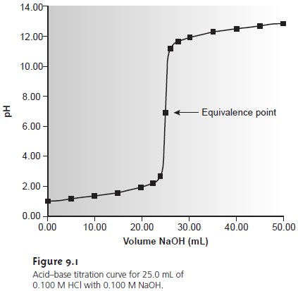
To find the end point we monitor some property of the titration reaction that has a well-defined value at the equivalence point. For example, the equivalence point for a titration of HCl with NaOH occurs at a pH of 7.0. We can find the end point, therefore, by monitoring the pH with a pH electrode or by adding an indicator that changes color at a pH of 7.0.

Suppose that the only available indicator changes color at a pH of 6.8. Is this end point close enough to the equivalence point that the titration error may be safely ignored? To answer this question we need to know how the pH changes dur- ing the titration.

A titration curve provides us with a visual picture of how a property, such as pH, changes as we add titrant (Figure 9.1). We can measure this titration curve ex- perimentally by suspending a pH electrode in the solution containing the analyte, monitoring the pH as titrant is added. As we will see later, we can also calculate the expected titration curve by considering the reactions responsible for the change in pH. However we arrive at the titration curve, we may use it to evaluate an indica- tor’s likely titration error. For example, the titration curve in Figure 9.1 shows us that an end point pH of 6.8 produces a small titration error. Stopping the titration at an end point pH of 11.6, on the other hand, gives an unacceptably large titration error.

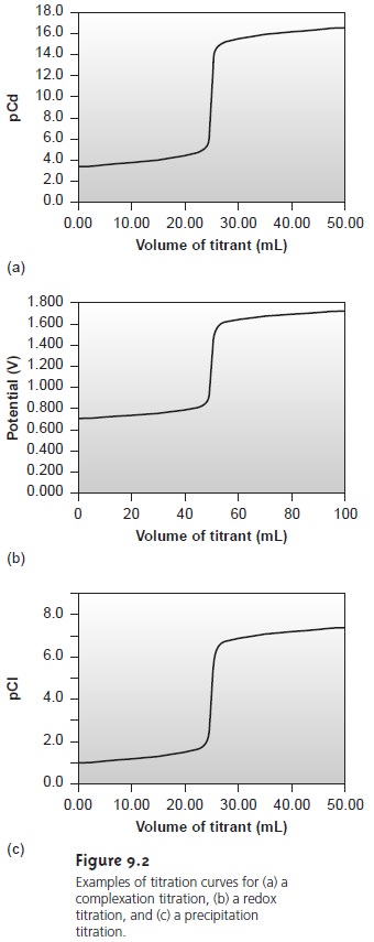
The titration curve in Figure 9.1 is not unique to an acid–base titration. Any titration curve that follows the change in concentration of a species in the titration reaction (plotted logarithmically) as a function of the volume of titrant has the same general sigmoidal shape. Several additional examples are shown in Figure 9.2.

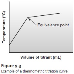
Concentration is not the only property that may be used to construct a titration curve. Other parameters, such as temperature or the absorbance of light, may be used if they show a significant change in value at the equivalence point. Many titra- tion reactions, for example, are exothermic. As the titrant and analyte react, the temperature of the system steadily increases. Once the titration is complete, further additions of titrant do not produce as exothermic a response, and the change in temperature levels off. A typical titration curve of temperature versus volume of titrant is shown in Figure 9.3. The titration curve contains two linear segments, the intersection of which marks the equivalence point.

The Buret

The only essential piece of equipment for an acid–base titration is a means for deliv- ering the titrant to the solution containing the analyte. The most common method for delivering the titrant is a buret (Figure 9.4). A buret is a long, narrow tube with graduated markings, and a stopcock for dispensing the titrant. Using a buret with a small internal diameter provides a better defined meniscus, making it easier to read the buret’s volume precisely. Burets are available in a variety of sizes and tolerances

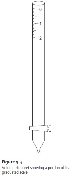
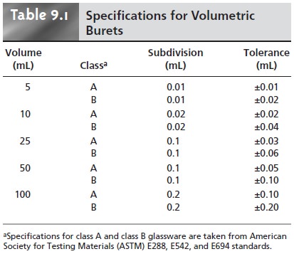
(Table 9.1), with the choice of buret determined by the demands of the analysis. The accuracy obtainable with a buret can be improved by calibrating it over several intermediate ranges of volumes using the same method described for calibrating pipets. In this manner, the volume of titrant delivered can be corrected for any variations in the buret’s internal diameter.

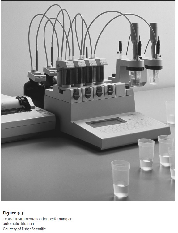
Titrations may be automated using a pump to deliver the titrant at a constant flow rate, and a solenoid valve to control the flow (Figure 9.5). The volume of titrant delivered is determined by multiplying the flow rate by the elapsed time. Au- tomated titrations offer the additional advantage of using a microcomputer for data storage and analysis.