Optimizing the Experimental Procedure: Response Surfaces

Response Surfaces

One of the most effective ways to think about optimization is to visualize how a sys- tem’s response changes when we increase or decrease the levels of one or more of its factors. A plot of the system’s response as a function of the factor levels is called a response surface. The simplest response surface is for a system with only one fac- tor. In this case the response surface is a straight or curved line in two dimensions. A calibration curve, such as that shown in Figure 14.1, is an example of a one-factor response surface in which the response (absorbance) is plotted on the y-axis versus the factor level (concentration of analyte) on the x-axis. Response surfaces can also be expressed mathematically. 

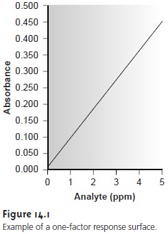
The response surface in Figure 14.1, for example, is

A = 0.008 + 0.0896C_A

where A is the absorbance, and C_A is the analyte’s concentration in parts per million.

For a two-factor system, such as the quantitative analysis for vanadium described earlier, the response surface is a flat or curved plane plotted in three dimen- sions. For example, Figure 14.2a shows the response surface for a system obeying the equation

R = 3.0 – 0.30A + 0.020AB

where R is the response, and A and B are the factor levels. Alternatively, we may represent a two-factor response surface as a contour plot, in which contour lines in- dicate the magnitude of the response (Figure 14.2b).

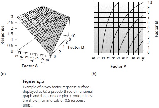
The response surfaces in Figure 14.2 are plotted for a limited range of factor levels (0 =< A =< 10, 0 =< B =< 10), but can be extended toward more positive or more negative values. This is an example of an unconstrained response surface. Most re- sponse surfaces of interest to analytical chemists, however, are naturally constrained by the nature of the factors or the response or are constrained by practical limits set by the analyst. The response surface in Figure 14.1, for example, has a natural con- straint on its factor since the smallest possible concentration for the analyte is zero. Furthermore, an upper limit exists because it is usually undesirable to extrapolate a calibration curve beyond the highest concentration standard.

If the equation for the response surface is known, then the optimum response is easy to locate. Unfortunately, the response surface is usually unknown; instead, its shape, and the location of the optimum response must be determined experimen- tally. The focus of this section is on useful experimental designs for optimizing ana- lytical methods. These experimental designs are divided into two broad categories: searching methods, in which an algorithm guides a systematic search for the opti- mum response; and modeling methods, in which we use a theoretical or empirical model of the response surface to predict the optimum response.