Open and Closed Hashing

Hashing

In this section, we consider a very efficient way to implement dictionaries. Recall that a dictionary is an abstract data type, namely, a set with the operations of searching (lookup), insertion, and deletion defined on its elements. The elements of this set can be of an arbitrary nature: numbers, characters of some alphabet, character strings, and so on. In practice, the most important case is that of records (student records in a school, citizen records in a governmental office, book records in a library).

Typically, records comprise several fields, each responsible for keeping a particular type of information about an entity the record represents. For example, a student record may contain fields for the student’s ID, name, date of birth, sex, home address, major, and so on. Among record fields there is usually at least one called a key that is used for identifying entities represented by the records (e.g., the student’s ID). In the discussion below, we assume that we have to implement a dictionary of n records with keys K₁, K₂, . . . , K_n.

Hashing is based on the idea of distributing keys among a one-dimensional array H [0..m − 1] called a hash table. The distribution is done by computing, for each of the keys, the value of some predefined function h called the hash function. This function assigns an integer between 0 and m − 1, called the hash address, to a key.

For example, if keys are nonnegative integers, a hash function can be of the form h(K) = K mod m; obviously, the remainder of division by m is always between 0 and m − 1. If keys are letters of some alphabet, we can first assign a letter its position in the alphabet, denoted here ord(K), and then apply the same kind of a function used for integers. Finally, if K is a character string 

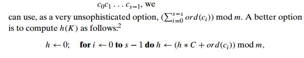
where C is a constant larger than every ord(c_i).

In general, a hash function needs to satisfy somewhat conflicting require-ments:

A hash table’s size should not be excessively large compared to the number of keys, but it should be sufficient to not jeopardize the implementation’s time efficiency (see below).

A hash function needs to distribute keys among the cells of the hash table as evenly as possible. (This requirement makes it desirable, for most applications, to have a hash function dependent on all bits of a key, not just some of them.) 

A hash function has to be easy to compute.

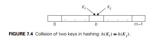
Obviously, if we choose a hash table’s size m to be smaller than the number of keys n, we will get collisions—a phenomenon of two (or more) keys being hashed into the same cell of the hash table (Figure 7.4). But collisions should be expected even if m is considerably larger than n (see Problem 5 in this section’s exercises). In fact, in the worst case, all the keys could be hashed to the same cell of the hash table. Fortunately, with an appropriately chosen hash table size and a good hash function, this situation happens very rarely. Still, every hashing scheme must have a collision resolution mechanism. This mechanism is different in the two principal versions of hashing: open hashing (also called separate chaining) and closed hashing (also called open addressing).

Open Hashing (Separate Chaining)

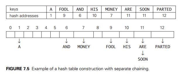
In open hashing, keys are stored in linked lists attached to cells of a hash table. Each list contains all the keys hashed to its cell. Consider, as an example, the following list of words:

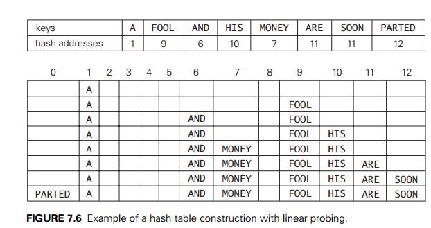
A, FOOL, AND, HIS, MONEY, ARE, SOON, PARTED.

As a hash function, we will use the simple function for strings mentioned above, i.e., we will add the positions of a word’s letters in the alphabet and compute the sum’s remainder after division by 13.

We start with the empty table. The first key is the word A; its hash value is h(A) = 1 mod 13 = 1. The second key—the word FOOL—is installed in the ninth cell since (6 + 15 + 15 + 12) mod 13 = 9, and so on. The final result of this process is given in Figure 7.5; note a collision of the keys ARE and SOON because h(ARE) = (1 + 18 + 5) mod 13 = 11 and h(SOON) = (19 + 15 + 15 + 14) mod 13 = 11.

How do we search in a dictionary implemented as such a table of linked lists? We do this by simply applying to a search key the same procedure that was used for creating the table. To illustrate, if we want to search for the key KID in the hash table of Figure 7.5, we first compute the value of the same hash function for the key: h(KID) = 11. Since the list attached to cell 11 is not empty, its linked list may contain the search key. But because of possible collisions, we cannot tell whether this is the case until we traverse this linked list. After comparing the string KID first with the string ARE and then with the string SOON, we end up with an unsuccessful search.

In general, the efficiency of searching depends on the lengths of the linked lists, which, in turn, depend on the dictionary and table sizes, as well as the quality

of the hash function. If the hash function distributes n keys among m cells of the hash table about evenly, each list will be about n/m keys long. The ratio α = n/m, called the load factor of the hash table, plays a crucial role in the efficiency of hashing. In particular, the average number of pointers (chain links) inspected in successful searches, S, and unsuccessful searches, U, turns out to be

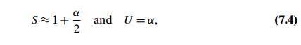
respectively, under the standard assumptions of searching for a randomly selected element and a hash function distributing keys uniformly among the table’s cells. These results are quite natural. Indeed, they are almost identical to searching sequentially in a linked list; what we have gained by hashing is a reduction in average list size by a factor of m, the size of the hash table.

Normally, we want the load factor to be not far from 1. Having it too small would imply a lot of empty lists and hence inefficient use of space; having it too large would mean longer linked lists and hence longer search times. But if we do have the load factor around 1, we have an amazingly efficient scheme that makes it possible to search for a given key for, on average, the price of one or two comparisons! True, in addition to comparisons, we need to spend time on computing the value of the hash function for a search key, but it is a constant-time operation, independent from n and m. Note that we are getting this remarkable efficiency not only as a result of the method’s ingenuity but also at the expense of extra space.

The two other dictionary operations—insertion and deletion—are almost identical to searching. Insertions are normally done at the end of a list (but see Problem 6 in this section’s exercises for a possible modification of this rule). Deletion is performed by searching for a key to be deleted and then removing it from its list. Hence, the efficiency of these operations is identical to that of searching, and they are all (1) in the average case if the number of keys n is about equal to the hash table’s size m.

Closed Hashing (Open Addressing)

In closed hashing, all keys are stored in the hash table itself without the use of linked lists. (Of course, this implies that the table size m must be at least as large as the number of keys n.) Different strategies can be employed for collision resolution. The simplest one—called linear probing—checks the cell following the one where the collision occurs. If that cell is empty, the new key is installed there; if the next cell is already occupied, the availability of that cell’s immediate successor is checked, and so on. Note that if the end of the hash table is reached, the search is wrapped to the beginning of the table; i.e., it is treated as a circular array. This method is illustrated in Figure 7.6 with the same word list and hash function used above to illustrate separate chaining.

To search for a given key K, we start by computing h(K) where h is the hash function used in the table construction. If the cell h(K) is empty, the search is unsuccessful. If the cell is not empty, we must compare K with the cell’s occupant: if they are equal, we have found a matching key; if they are not, we compare K with a key in the next cell and continue in this manner until we encounter either a matching key (a successful search) or an empty cell (unsuccessful search). For example, if we search for the word LIT in the table of Figure 7.6, we will get h(LIT) = (12 + 9 + 20) mod 13 = 2 and, since cell 2 is empty, we can stop immediately. However, if we search for KID with h(KID) = (11 + 9 + 4) mod 13 = 11, we will have to compare KID with ARE, SOON, PARTED, and A before we can declare the search unsuccessful.

Although the search and insertion operations are straightforward for this version of hashing, deletion is not. For example, if we simply delete the key ARE from the last state of the hash table in Figure 7.6, we will be unable to find the key SOON afterward. Indeed, after computing h(SOON) = 11, the algorithm would find this location empty and report the unsuccessful search result. A simple solution

is to use “lazy deletion,” i.e., to mark previously occupied locations by a special symbol to distinguish them from locations that have not been occupied.

The mathematical analysis of linear probing is a much more difficult problem than that of separate chaining. The simplified versions of these results state that the average number of times the algorithm must access the hash table with the load factor α in successful and unsuccessful searches is, respectively,

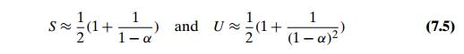
(and the accuracy of these approximations increases with larger sizes of the hash table). These numbers are surprisingly small even for densely populated tables, i.e., for large percentage values of α:

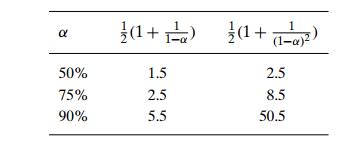
Still, as the hash table gets closer to being full, the performance of linear prob-ing deteriorates because of a phenomenon called clustering. A cluster in linear probing is a sequence of contiguously occupied cells (with a possible wrapping). For example, the final state of the hash table of Figure 7.6 has two clusters. Clus-ters are bad news in hashing because they make the dictionary operations less efficient. As clusters become larger, the probability that a new element will be attached to a cluster increases; in addition, large clusters increase the probabil-ity that two clusters will coalesce after a new key’s insertion, causing even more clustering.

Several other collision resolution strategies have been suggested to alleviate this problem. One of the most important is double hashing. Under this scheme, we use another hash function, s(K), to determine a fixed increment for the probing sequence to be used after a collision at location l = h(K):

(l + s(K)) mod m,                   (l + 2s(K)) mod m,             . . . .       (7.6)

To guarantee that every location in the table is probed by sequence (7.6), the incre-ment s(k) and the table size m must be relatively prime, i.e., their only common divisor must be 1. (This condition is satisfied automatically if m itself is prime.) Some functions recommended in the literature are s(k) = m − 2 − k mod (m − 2) and s(k) = 8 − (k mod 8) for small tables and s(k) = k mod 97 + 1 for larger ones.

Mathematical analysis of double hashing has proved to be quite difficult. Some partial results and considerable practical experience with the method suggest that with good hashing functions—both primary and secondary—double hashing is su-perior to linear probing. But its performance also deteriorates when the table gets close to being full. A natural solution in such a situation is rehashing: the current table is scanned, and all its keys are relocated into a larger table.

It is worthwhile to compare the main properties of hashing with balanced search trees—its principal competitor for implementing dictionaries.

Asymptotic time efficiency With hashing, searching, insertion, and deletion can be implemented to take  (1) time on the average but  (n) time in the very unlikely worst case. For balanced search trees, the average time efficiencies are  (log n) for both the average and worst cases.

Ordering preservation Unlike balanced search trees, hashing does not assume existence of key ordering and usually does not preserve it. This makes hashing less suitable for applications that need to iterate over the keys in or-der or require range queries such as counting the number of keys between some lower and upper bounds.

Since its discovery in the 1950s by IBM researchers, hashing has found many important applications. In particular, it has become a standard technique for stor-ing a symbol table—a table of a computer program’s symbols generated during compilation. Hashing is quite handy for such AI applications as checking whether positions generated by a chess-playing computer program have already been con-sidered. With some modifications, it has also proved to be useful for storing very large dictionaries on disks; this variation of hashing is called extendible hashing. Since disk access is expensive compared with probes performed in the main mem-ory, it is preferable to make many more probes than disk accesses. Accordingly, a location computed by a hash function in extendible hashing indicates a disk ad-dress of a bucket that can hold up to b keys. When a key’s bucket is identified, all its keys are read into main memory and then searched for the key in question. In the next section, we discuss B-trees, a principal alternative for storing large dictionaries.

Exercises 7.3

            For the input 30, 20, 56, 75, 31, 19 and hash function h(K) = K mod 11

            construct the open hash table.

            find the largest number of key comparisons in a successful search in this table.

            find the average number of key comparisons in a successful search in this table.

            For the input 30, 20, 56, 75, 31, 19 and hash function h(K) = K mod 11

construct the closed hash table.

            find the largest number of key comparisons in a successful search in this table.

            find the average number of key comparisons in a successful search in this table.

            Why is it not a good idea for a hash function to depend on just one letter (say, the first one) of a natural-language word?

            Find the probability of all n keys being hashed to the same cell of a hash table of size m if the hash function distributes keys evenly among all the cells of the table.

            Birthday paradox The birthday paradox asks how many people should be in a room so that the chances are better than even that two of them will have the same birthday (month and day). Find the quite unexpected answer to this problem. What implication for hashing does this result have?

            Answer the following questions for the separate-chaining version of hashing.

            Where would you insert keys if you knew that all the keys in the dictionary are distinct? Which dictionary operations, if any, would benefit from this modification?

            We could keep keys of the same linked list sorted. Which of the dictio-nary operations would benefit from this modification? How could we take advantage of this if all the keys stored in the entire table need to be sorted?

            Explain how to use hashing to check whether all elements of a list are distinct. What is the time efficiency of this application? Compare its efficiency with that of the brute-force algorithm (Section 2.3) and of the presorting-based algorithm (Section 6.1).

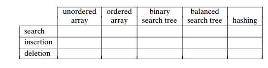
            Fill in the following table with the average-case (as the first entry) and worst-case (as the second entry) efficiency classes for the five implementations of the ADT dictionary:

            We have discussed hashing in the context of techniques based on space–time trade-offs. But it also takes advantage of another general strategy. Which one?

Write a computer program that uses hashing for the following problem. Given a natural-language text, generate a list of distinct words with the number of occurrences of each word in the text. Insert appropriate counters in the pro-gram to compare the empirical efficiency of hashing with the corresponding theoretical results.