Nyquist Plot

Nyquist Plot:

The Nyquist plot is a polar plot of the function

The Nyquist stability criterion relates the location of the roots of the characteristic equation to the open-loop frequency response of the system. In this, the computation of closed-loop poles is not necessary to determine the stability of the system and the stability study can be carried out graphically from the open-loop frequency response. Therefore experimentally determined open-loop frequency response can be used directly for the study of stability. When the feedback path is closed. The Nyquist criterion has the following features that make it an alternative method that is attractive for the analysis and design of control systems. 1. In addition to providing information on absolute and relative.

Nyquist Plot Example

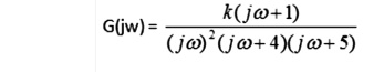
Consider the following transfer function

Change it from “s” domain to “jw” domain:

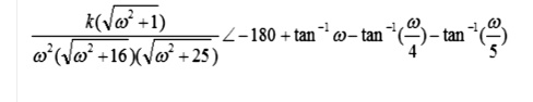
Find the magnitude and phase angle equations:

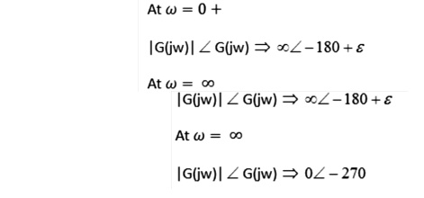
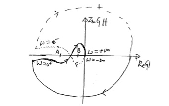
Evaluate magnitude and phase angle at ω= 0+ and ω = +∞

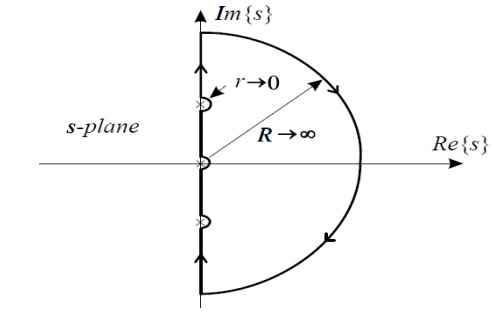
Draw the nyquist plot:

Frequency domain specifications

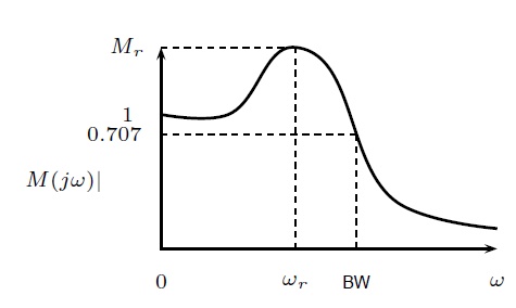
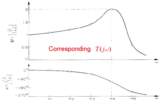
The resonant peak Mr is the maximum value of jM(jw)j.

The resonant frequency !r is the frequency at which the peak resonance Mr occurs.

The bandwidth BW is the frequency at which(jw) drops to 70:7% (3 dB) of its zero-frequency value.

Mr indicates the relative stability of a stable closed loop system.

A large Mr corresponds to larger maximum overshoot of the step response. Desirable value: 1.1 to 1.5

BW gives an indication of the transient response properties of a control system.

A large bandwidth corresponds to a faster rise time. BW and rise time tr are inversely proportional.

BW also indicates the noise-filtering characteristics and robustness of the system. Increasing wn increases BW.

BW and Mr are proportional to each other.

Constant M and N circles

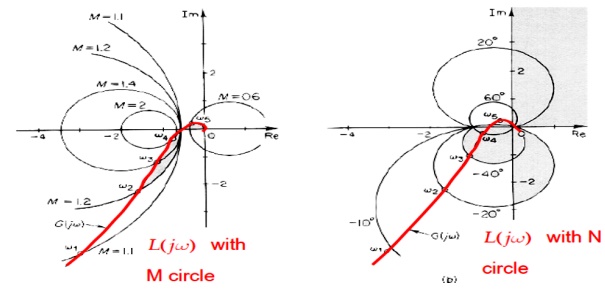
Consider a candidate design of a loop transfer function L( jω) shown on the RHS.

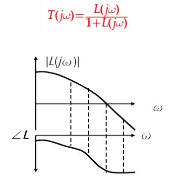
Evaluate T( jω) from L( jω) in the manner of frequency point by frequency point.

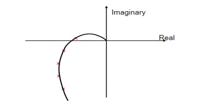
Alternatively, the Bode plot of L( jω) can also be show on the complex plane to form its Nyquist plot.

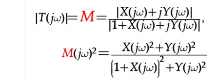
M circles (constant magnitude of T)

In order to precisely evaluate |T( jω)| from the Nyquist plot of L( jω), a tool called M circle is developed as followed.

Let L( jω)=X+jY, where X is the real and Y the imaginary part . Then

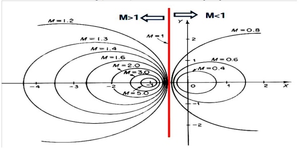
Rearranging the above equations, it gives X2(1-M2)-2M2X-M2+(1-M2)Y2 = 0

That is, all (X, Y) pair corresponding to a constant value of M for a circle on the complex plane. Therefore, we have the following (constant) M circles on the complex plane as shown below.

Similarly, it can be shown that the phase of T( jω) be

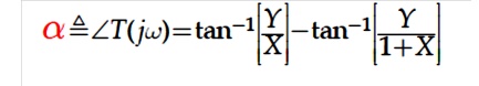
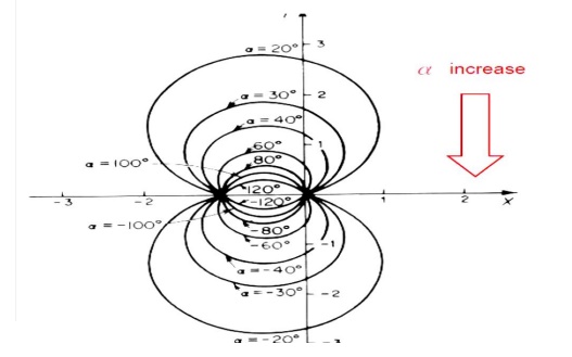
It can be shown that all (X, Y) pair which corresponds to the same constant phase of T (i.e., constant N) forms a circle on the complex plane as shown below.

Example

Nyquist plot of L( jω), and M-N circles of T( jω)

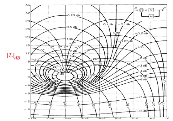
Nichols Chart

The Nyquist plot of L( jω) can also be represented by its polar form using dB as magnitude and degree as phase.

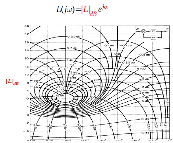
And ll L( jω) which corresponds to a constant α( jω) can be draw as a locus of M circle on this plane as shown below.

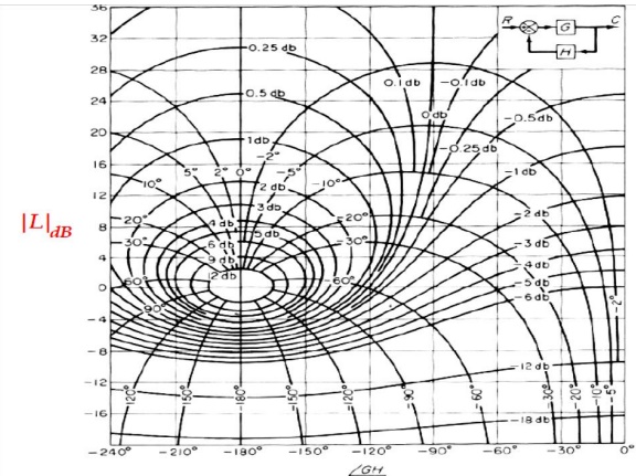
Combining the above two graphs of M circles and N circles, we have the Nicholas chart below.