Lower-Bound Arguments

Lower-Bound Arguments

We can look at the efficiency of an algorithm two ways. We can establish its asymp-totic efficiency class (say, for the worst case) and see where this class stands with respect to the hierarchy of efficiency classes outlined in Section 2.2. For exam-ple, selection sort, whose efficiency is quadratic, is a reasonably fast algorithm, whereas the algorithm for the Tower of Hanoi problem is very slow because its ef-ficiency is exponential. We can argue, however, that this comparison is akin to the proverbial comparison of apples to oranges because these two algorithms solve different problems. The alternative and possibly “fairer” approach is to ask how efficient a particular algorithm is with respect to other algorithms for the same problem. Seen in this light, selection sort has to be considered slow because there are O(n log n) sorting algorithms; the Tower of Hanoi algorithm, on the other hand, turns out to be the fastest possible for the problem it solves.

When we want to ascertain the efficiency of an algorithm with respect to other algorithms for the same problem, it is desirable to know the best possible efficiency any algorithm solving the problem may have. Knowing such a lower bound can tell us how much improvement we can hope to achieve in our quest for a better algorithm for the problem in question. If such a bound is tight, i.e., we already know an algorithm in the same efficiency class as the lower bound, we can hope for a constant-factor improvement at best. If there is a gap between the efficiency of the fastest algorithm and the best lower bound known, the door for possible improvement remains open: either a faster algorithm matching the lower bound could exist or a better lower bound could be proved.

In this section, we present several methods for establishing lower bounds and illustrate them with specific examples. As we did in analyzing the efficiency of specific algorithms in the preceding chapters, we should distinguish between a lower-bound class and a minimum number of times a particular operation needs to be executed. As a rule, the second problem is more difficult than the first. For example, we can immediately conclude that any algorithm for finding the median of n numbers must be in  (n) (why?), but it is not simple at all to prove that any comparison-based algorithm for this problem must do at least 3(n − 1)/2 comparisons in the worst case (for odd n).

Trivial Lower Bounds

The simplest method of obtaining a lower-bound class is based on counting the number of items in the problem’s input that must be processed and the number of output items that need to be produced. Since any algorithm must at least “read” all the items it needs to process and “write” all its outputs, such a count yields a trivial lower bound. For example, any algorithm for generating all permutations of n distinct items must be in  (n!) because the size of the output is n!. And this bound is tight because good algorithms for generating permutations spend a constant time on each of them except the initial one (see Section 4.3).

As another example, consider the problem of evaluating a polynomial of degree n

p(x) = a_nxⁿ + a_n−1xⁿ⁻¹ + ^{. . .} + a₀

at a given point x, given its coefficients a_n, a_n−1, . . . , a₀. It is easy to see that all the coefficients have to be processed by any polynomial-evaluation algorithm. Indeed, if it were not the case, we could change the value of an unprocessed coefficient, which would change the value of the polynomial at a nonzero point x. This means that any such algorithm must be in  (n). This lower bound is tight because both the right-to-left evaluation algorithm (Problem 2 in Exercises 6.5) and Horner’s rule (Section 6.5) are both linear.

In a similar vein, a trivial lower bound for computing the product of two n × n matrices is  (n²) because any such algorithm has to process 2n² elements in the input matrices and generate n² elements of the product. It is still unknown, however, whether this bound is tight.

Trivial lower bounds are often too low to be useful. For example, the trivial bound for the traveling salesman problem is  (n²), because its input is n(n − 1)/2 intercity distances and its output is a list of n + 1 cities making up an optimal tour. But this bound is all but useless because there is no known algorithm with the running time being a polynomial function of any degree.

There is another obstacle to deriving a meaningful lower bound by this method. It lies in determining which part of an input must be processed by any algorithm solving the problem in question. For example, searching for an ele-ment of a given value in a sorted array does not require processing all its elements (why?). As another example, consider the problem of determining connectivity of an undirected graph defined by its adjacency matrix. It is plausible to expect that any such algorithm would have to check the existence of each of the n(n − 1)/2 potential edges, but the proof of this fact is not trivial.

Informatikon-Theoretic Arguments

While the approach outlined above takes into account the size of a problem’s output, the information-theoretical approach seeks to establish a lower bound based on the amount of information it has to produce. Consider, as an example, the well-known game of deducing a positive integer between 1 and n selected by somebody by asking that person questions with yes/no answers. The amount of uncertainty that any algorithm solving this problem has to resolve can be measured by log₂ n , the number of bits needed to specify a particular number among the n possibilities. We can think of each question (or, to be more accurate, an answer to each question) as yielding at most 1 bit of information about the algorithm’s output, i.e., the selected number. Consequently, any such algorithm will need at least log₂ n such steps before it can determine its output in the worst case.

The approach we just exploited is called the information-theoretic argument because of its connection to information theory. It has proved to be quite useful for finding the so-called information-theoretic lower bounds for many problems involving comparisons, including sorting and searching. Its underlying idea can be realized much more precisely through the mechanism of decision trees. Because of the importance of this technique, we discuss it separately and in more detail in Section 11.2.

Adversary Arguments

Let us revisit the same game of “guessing” a number used to introduce the idea of an information-theoretic argument. We can prove that any algorithm that solves this problem must ask at least log₂ n questions in its worst case by playing the role of a hostile adversary who wants to make an algorithm ask as many questions as possible. The adversary starts by considering each of the numbers between 1 and n as being potentially selected. (This is cheating, of course, as far as the game is concerned, but not as a way to prove our assertion.) After each question, the adversary gives an answer that leaves him with the largest set of numbers consistent with this and all the previously given answers. This strategy leaves him with at least one-half of the numbers he had before his last answer. If an algorithm stops before the size of the set is reduced to 1, the adversary can exhibit a number that could be a legitimate input the algorithm failed to identify. It is a simple technical matter now to show that one needs log₂ n iterations to shrink an n-element set to a one-element set by halving and rounding up the size of the remaining set. Hence, at least log₂ n questions need to be asked by any algorithm in the worst case.

This example illustrates the adversary method for establishing lower bounds. It is based on following the logic of a malevolent but honest adversary: the malev- olence makes him push the algorithm down the most time-consuming path, and his honesty forces him to stay consistent with the choices already made. A lower bound is then obtained by measuring the amount of work needed to shrink a set of potential inputs to a single input along the most time-consuming path.

As another example, consider the problem of merging two sorted lists of size n

a₁ < a₂ < ^{. . .} < a_n              and b₁ < b₂ < ^{. . .} < b_n

into a single sorted list of size 2n. For simplicity, we assume that all the a’s and b’s are distinct, which gives the problem a unique solution. We encountered this problem when discussing mergesort in Section 5.1. Recall that we did merging by repeatedly comparing the first elements in the remaining lists and outputting the smaller among them. The number of key comparisons in the worst case for this algorithm for merging is 2n − 1.

Is there an algorithm that can do merging faster? The answer turns out to be no. Knuth [KnuIII, p. 198] quotes the following adversary method for proving that 2n − 1 is a lower bound on the number of key comparisons made by any comparison-based algorithm for this problem. The adversary will employ the following rule: reply true to the comparison a_i < b_j if and only if i < j. This will force any correct merging algorithm to produce the only combined list consistent with this rule:

b₁ < a₁ < b₂ < a₂ < ^{. . .} < b_n < a_n.

To produce this combined list, any correct algorithm will have to explicitly com-pare 2n − 1 adjacent pairs of its elements, i.e., b₁ to a₁, a₁ to b₂, and so on. If one of these comparisons has not been made, e.g., a₁ has not been compared to b₂, we can transpose these keys to get

b₁ < b₂ < a₁ < a₂ < ^{. . .} < b_n < a_n,

which is consistent with all the comparisons made but cannot be distinguished from the correct configuration given above. Hence, 2n − 1 is, indeed, a lower bound for the number of key comparisons needed for any merging algorithm.

Problem Reduction

We have already encountered the problem-reduction approach in Section 6.6. There, we discussed getting an algorithm for problem P by reducing it to another problem Q solvable with a known algorithm. A similar reduction idea can be used for finding a lower bound. To show that problem P is at least as hard as another problem Q with a known lower bound, we need to reduce Q to P (not P to Q!). 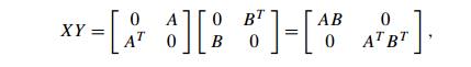In other words, we should show that an arbitrary instance of problem Q can be transformed (in a reasonably efficient fashion) to an instance of problem P , so any algorithm solving P would solve Q as well. Then a lower bound for Q will be a lower bound for P . Table 11.1 lists several important problems that are often used for this purpose.

We will establish the lower bounds for sorting and searching in the next sec-tion. The element uniqueness problem asks whether there are duplicates among n given numbers. (We encountered this problem in Sections 2.3 and 6.1.) The proof of the lower bound for this seemingly simple problem is based on a very sophisti-cated mathematical analysis that is well beyond the scope of this book (see, e.g., [Pre85] for a rather elementary exposition). As to the last two algebraic prob-lems in Table 11.1, the lower bounds quoted are trivial, but whether they can be improved remains unknown.

As an example of establishing a lower bound by reduction, let us consider the Euclidean minimum spanning tree problem: given n points in the Cartesian plane, construct a tree of minimum total length whose vertices are the given points. As a problem with a known lower bound, we use the element uniqueness problem. We can transform any set x₁, x ₂, . . . , x_n of n real numbers into a set of n points in the Cartesian plane by simply adding 0 as the points’ y coordinate: (x₁, 0), (x₂, 0), . . . , (x_n, 0). Let T be a minimum spanning tree found for this set of points. Since T must contain a shortest edge, checking whether T contains a zero-length edge will answer the question about uniqueness of the given numbers. This reduction implies that  (n log n) is a lower bound for the Euclidean minimum spanning tree problem, too.

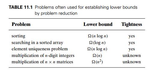
Since the final results about the complexity of many problems are not known, the reduction technique is often used to compare the relative complexity of prob-lems. For example, the formulas

show that the problems of computing the product of two n-digit integers and squaring an n-digit integer belong to the same complexity class, despite the latter being seemingly simpler than the former.

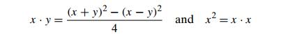
There are several similar results for matrix operations. For example, multi-plying two symmetric matrices turns out to be in the same complexity class as multiplying two arbitrary square matrices. This result is based on the observation that not only is the former problem a special case of the latter one, but also that we can reduce the problem of multiplying two arbitrary square matrices of order n, say, A and B, to the problem of multiplying two symmetric matrices

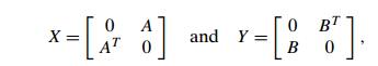
where A^T and B^T are the transpose matrices of A and B (i.e., A^T [i, j ] = A[j, i] and B^T [i, j ] = B[j, i]), respectively, and 0 stands for the n × n matrix whose elements are all zeros. Indeed,

from which the needed product AB can be easily extracted. (True, we will have to multiply matrices twice the original size, but this is just a minor technical complication with no impact on the complexity classes.)

Though such results are interesting, we will encounter even more important applications of the reduction approach to comparing problem complexity in Sec-tion 11.3.

Exercises 11.1

            Prove that any algorithm solving the alternating-disk puzzle (Problem 14 in Exercises 3.1) must make at least n(n + 1)/2 moves to solve it. Is this lower bound tight?

            Prove that the classic recursive algorithm for the Tower of Hanoi puzzle (Section 2.4) makes the minimum number of disk moves needed to solve the problem.

            Find a trivial lower-bound class for each of the following problems and indi-cate, if you can, whether this bound is tight.

            finding the largest element in an array

            checking completeness of a graph represented by its adjacency matrix

            generating all the subsets of an n-element set

            determining whether n given real numbers are all distinct

            Consider the problem of identifying a lighter fake coin among n identical-looking coins with the help of a balance scale. Can we use the same information-theoretic argument as the one in the text for the number of ques-tions in the guessing game to conclude that any algorithm for identifying the fake will need at least log₂ n weighings in the worst case?

Prove that any comparison-based algorithm for finding the largest element of an n-element set of real numbers must make n − 1 comparisons in the worst case.

            Find a tight lower bound for sorting an array by exchanging its adjacent elements.

            Give an adversary-argument proof that the time efficiency of any algorithm that checks connectivity of a graph with n vertices is in  (n²), provided the only operation allowed for an algorithm is to inquire about the presence of an edge between two vertices of the graph. Is this lower bound tight?

            What is the minimum number of comparisons needed for a comparison-based sorting algorithm to merge any two sorted lists of sizes n and n + 1 elements, respectively? Prove the validity of your answer.

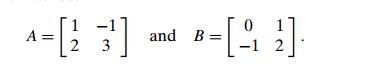
Find the product of matrices A and B through a transformation to a product of two symmetric matrices if

            a. Can one use this section’s formulas that indicate the complexity equiva-lence of multiplication and squaring of integers to show the complexity equivalence of multiplication and squaring of square matrices?

                                                                            Show that multiplication of two matrices of order n can be reduced to squaring a matrix of order 2n.

            Find a tight lower-bound class for the problem of finding two closest numbers among n real numbers x₁, x₂, . . . , x_n.

            Find a tight lower-bound class for the number placement problem (Problem 9 in Exercises 6.1).