Implementation of tree search using MPI and dynamic partitioning

Implementation of tree search using MPI and dynamic partitioning

In an MPI program that dynamically partitions the search tree, we can try to emu-late the dynamic partitioning that we used in the Pthreads and OpenMP programs. Recall that in those programs, before each pass through the main while loop in the search function, a thread called a boolean-valued function called Terminated. When a thread ran out of work—that is, its stack was empty—it went into a condition wait (Pthreads) or a busy-wait (OpenMP) until it either received additional work or it was notified that there was no more work. In the first case, it returned to searching for a best tour. In the second case, it quit. A thread that had at least two records on its stack would give half of its stack to one of the waiting threads.

Much of this can be emulated in a distributed-memory setting. When a process runs out of work, there’s no condition wait, but it can enter a busy-wait, in which it waits to either receive more work or notification that the program is terminat-ing. Similarly, a process with work can split its stack and send work to an idle process.

The key difference is that there is no central repository of information on which processes are waiting for work, so a process that splits its stack can’t just dequeue a queue of waiting processes or call a function such as pthread_cond_signal. It needs to “know” a process that’s waiting for work so it can send the waiting process more work. Thus, rather than simply going into a busy-wait for additional work or termination, a process that has run out of work should send a request for work to another process. If it does this, then, when a process enters the Terminated func-tion, it can check to see if there’s a request for work from some other process. If there is, and the process that has just entered Terminated has work, it can send part of its stack to the requesting process. If there is a request, and the process has no work available, it can send a rejection. Thus, when we have distributed-memory, pseudocode for our Terminated function can look something like the pseudocode shown in Program 6.10.

Terminated begins by checking on the number of tours that the process has in its stack (Line 1); if it has at least two that are “worth sending,” it calls Fulfill_request (Line 2). Fulfill_request checks to see if the process has received a request for work. If it has, it splits its stack and sends work to the requesting process. If it hasn’t received a request, it just returns. In either case, when it returns from Fulfill_request it returns from Terminated and continues searching.

If the calling process doesn’t have at least two tours worth sending, Terminated calls Send rejects (Line 5), which checks for any work requests from other processes and sends a “no work” reply to each requesting process. After this, Terminated checks to see if the calling process has any work at all. If it does—that is, if its stack isn’t empty—it returns and continues searching.

Things get interesting when the calling process has no work left (Line 9). If there’s only one process in the communicator (comm sz D 1), then the process returns from Terminated and quits. If there’s more than one process, then the process “announces” that it’s out of work in Line 11. This is part of the implementation

Program 6.10: Terminated function for a dynamically partitioned TSP solver that uses MPI

          if (My_avail_tour_count(my_stack) >= 2) {

          Fulfill_request(my_stack);

          return false;  /*  Still more work * /

          } else { /*  At most 1 available tour  */

          Send rejects();  /*  Tell everyone who’s requested          */

          /*       work that I have none    */

          if (!Empty_stack(my_stack)) {

          return false;  /*  Still more work  */

          } else {  /*  Empty stack  */

          if (comm_sz == 1) return true;

          Out_of_work();

          work request sent = false;

          while (1) {

          Clear msgs();  /*  Msgs unrelated to work, termination  */

          if (No_work_left()) {

          return true;  /  No work left.  Quit  /

          } else if (!work_request_sent) {

          Send_work_request();    /*       Request work from someone   */

          work_request_sent = true;

          } else {

          Check_for_work(&work_request_sent, &work_avail);

          if (work_avail) {

          Receive_work(my_stack);

          return false;

          }

          }

          }  /*  while  */

          } /*  Empty stack  */

          } /*  At most 1 available tour  */

of a “distributed termination detection algorithm,” which we’ll discuss shortly. For now, let’s just note that the termination detection algorithm that we used with shared-memory may not work, since it’s impossible to guarantee that a variable storing the number of processes that have run out of work is up to date.

Before entering the apparently infinite while loop (Line 13), we set the variable work_request_sent to false (Line 12). As its name suggests, this variable tells us whether we’ve sent a request for work to another process; if we have, we know that we should wait for work or a message saying “no work available” from that process before sending out a request to another process.

The while(1) loop is the distributed-memory version of the OpenMP busy-wait loop. We are essentially waiting until we either receive work from another process or we receive word that the search has been completed.

When we enter the while(1) loop, we deal with any outstanding messages in Line 14. We may have received updates to the best tour cost and we may have received requests for work. It’s essential that we tell processes that have requested work that we have none, so that they don’t wait forever when there’s no work avail-able. It’s also a good idea to deal with updates to the best tour cost, since this will free up space in the sending process’ message buffer.

After clearing out outstanding messages, we iterate through the possibilities:

The search has been completed, in which case we quit (Lines 15–16).

We don’t have an outstanding request for work, so we choose a process and send it a request (Lines 17–19). We’ll take a closer look at the problem of which process should be sent a request shortly.

We do have an outstanding request for work (Lines 21–25). So we check whether the request has been fulfilled or rejected. If it has been fulfilled, we receive the new work and return to searching. If we received a rejection, we set

work_request sent to false and continue in the loop. If the request was neither fulfilled nor rejected, we also continue in the while(1) loop.

Let’s take a closer look at some of these functions.

My_avail_tour_count

The function My_avail_tour count can simply return the size of the process’ stack. It can also make use of a “cutoff length.” When a partial tour has already visited most of the cities, there will be very little work associated with the subtree rooted at the partial tour. Since sending a partial tour is likely to be a relatively expensive operation, it may make sense to only send partial tours with fewer than some cutoff number of edges. In Exercise 6.24 we take a look at how such a cutoff affects the overall run-time of the program.

Fulfill_request

If a process has enough work so that it can usefully split its stack, it calls Fulfill_request (Line 2). Fulfill_request uses MPI Iprobe to check for a request for work from another process. If there is a request, it receives it, splits its stack, and sends work to the requesting process. If there isn’t a request for work, the process just returns.

Splitting the stack

A Split_stack function is called by Fulfill_request. It uses the same basic algo-rithm as the Pthreads and OpenMP functions, that is, alternate partial tours with fewer than split_cutoff cities are collected for sending to the process that has requested work. However, in the shared-memory programs, we simply copy the tours (which are pointers) from the original stack to a new stack. Unfortunately, because of the pointers involved in the new stack, such a data structure cannot be simply sent to another process (see Exercise 6.25). Thus, the MPI version of Split_stack packs the contents of the new stack into contiguous memory and sends the block of contiguous memory, which is unpacked by the receiver into a new stack.

MPI provides a function, MPI_Pack, for packing data into a buffer of contiguous memory. It also provides a function, MPI Unpack, for unpacking data from a buffer of contiguous memory. We took a brief look at them in Exercise 6.20 of Chapter 3. Recall that their syntax is

int MPI_Pack(     

void* data_to_be_packed        /*       in       */,

int     to_be_packed_count      /*       in       */,

MPI_Datatype     datatype     /*       in       */,

void* contig_buf  /*       out    */,

int     contig_buf_size    /*       in       */,

int*    position_p  /*       in/out */,

MPI_Comm         comm          /*       in       */);

int MPI_Unpack(                             

 void*         contig_buf

int     contig_buf_size

int*    position_p

void* unpacked_data

int     unpack_count

MPI_Datatype     datatype

MPI_Comm         comm.

MPI_Pack takes the data in data to be packed and packs it into contig_buf. The *position_p argument keeps track of where we are in contig_buf. When the function is called, it should refer to the first available location in contig buf before data to be packed is added. When the function returns, it should refer to the first available location in contig_buf after data_to_be_packed has been added.

MPI Unpack reverses the process. It takes the data in contig buf and unpacks it into unpacked data. When the function is called, position p should refer to the first location in contig buf that hasn’t been unpacked. When it returns, position p should refer to the next location in contig buf after the data that was just unpacked.

As an example, suppose that a program contains the following definitions:

typedef struct       {       

int*  cities;  /*  Cities in partial tour  */

int count;    / * Number of cities in partial tour  */

int cost;       /*  Cost of partial tour   */

} tour_struct;                

typedef tour_struct*      tour_t;

Then we can send a variable with type tour t using the following code:

void Send_tour(tour_t tour, int dest) { int position = 0;

MPI_Pack(tour ->cities, n+1, MPI_INT, contig buf, LARGE, &position, comm);

MPI_Pack(&tour- >count, 1, MPI_INT, contig buf, LARGE, &position, comm);

MPI_Pack(&tour ->cost, 1, MPI_INT, contig buf, LARGE,

&position, comm);

MPI_Send(contig buf, position, MPI_PACKED, dest, 0, comm);

}        /*  Send tour  */

Similarly, we can receive a variable of type tour t using the following code:

void Receive_tour(tour_t tour, int src) {

int position = 0;

MPI Recv(contig_buf, LARGE, MPI_PACKED, src, 0, comm,

MPI_STATUS_IGNORE);

MPI_Unpack(contig_buf, LARGE, &position, tour->cities, n+1, MPI_INT, comm);

MPI Unpack(contig_buf, LARGE, &position, &tour ->count, 1, MPI_INT, comm);

MPI Unpack(contig_buf, LARGE, &position, &tour- >cost, 1, MPI_INT, comm);

          /*  Receive tour  */

Note that the MPI datatype that we use for sending and receiving packed buffers is

MPI_PACKED.

Send_rejects

The Send_rejects function (Line 5) is similar to the function that looks for new best tours. It uses MPI_Iprobe to search for messages that have requested work. Such messages can be identified by a special tag value, for example, WORK REQ TAG. When such a message is found, it’s received, and a reply is sent indicating that there is no work available. Note that both the request for work and the reply indicating there is no work can be messages with zero elements, since the tag alone informs the receiver of the message’s purpose. Even though such messages have no content outside of the envelope, the envelope does take space and they need to be received.

Distributed termination detection

The functions Out_of_work and No_work_left (Lines 11 and 15) implement the ter-mination detection algorithm. As we noted earlier, an algorithm that’s modeled on the termination detection algorithm we used in the shared-memory programs will have problems. To see this, suppose each process stores a variable oow, which stores the number of processes that are out of work. The variable is set to 0 when the program starts. Each time a process runs out of work, it sends a message to all the other pro-cesses saying it’s out of work so that all the processes will increment their copies of oow. 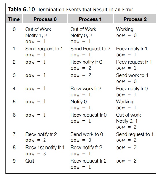Similarly, when a process receives work from another process, it sends a message to every process informing them of this, and each process will decrement its copy of oow. Now suppose we have three process, and process 2 has work but processes 0 and 1 have run out of work. Consider the sequence of events shown in Table 6.10.

The error here is that the work sent from process 1 to process 0 is lost. The rea-son is that process 0 receives the notification that process 2 is out of work before it receives the notification that process 1 has received work. This may seem improbable,

but it’s not improbable that process 1 was, for example, interrupted by the operating system and its message wasn’t transmitted until after the message from process 2 was transmitted.

Although MPI guarantees that two messages sent from process A to process B will, in general, be received in the order in which they were sent, it makes no guaran-tee about the order in which messages will be received if they were sent by different processes. This is perfectly reasonable in light of the fact that different processes will, for various reasons, work at different speeds.

Distributed termination detection is a challenging problem, and much work has gone into developing algorithms that are guaranteed to correctly detect it. Concep-tually, the simplest of these algorithms relies on keeping track of a quantity that is conserved and can be measured precisely. Let’s call it energy, since, of course, energy is conserved. At the start of the program, each process has 1 unit of energy. When a process runs out of work, it sends its energy to process 0. When a process fulfills a request for work, it divides its energy in half, keeping half for itself, and sending half to the process that’s receiving the work. Since energy is conserved and since the program started with comm_sz units, the program should terminate when process 0 finds that it has received a total of comm_sz units.

The Out of work function when executed by a process other than 0 sends its energy to process 0. Process 0 can just add its energy to a received_energy variable. The No_work_left function also depends on whether process 0 or some other process is calling. If process 0 is calling, it can receive any outstanding messages sent by

Out_of_work and add the energy into received energy. If received energy equals comm sz, process 0 can send a termination message (with a special tag) to every process. On the other hand, a process other than 0 can just check to see if there’s a message with the termination tag.

The tricky part here is making sure that no energy is inadvertently lost; if we try to use floats or doubles, we’ll almost certainly run into trouble since at some point dividing by two will result in underflow. Since the amount of energy in exact arithmetic can be represented by a common fraction, we can represent the amount of energy on each process exactly by a pair of fixed-point numbers. The denominator will always be a power of two, so we can represent it by its base-two logarithm. For a large problem it is possible that the numerator could overflow. However, if this becomes a problem, there are libraries that provide arbitrary precision rational numbers (e.g, GMP [21]). An alternate solution is explored in Exercise 6.26.

Sending requests for work

Once we’ve decided on which process we plan to send a request to, we can just send a zero-length message with a “request for work” tag. However, there are many possibilities for choosing a destination:

1. Loop through the processes in round-robin fashion. Start with (my rank + 1) % comm sz and increment this destination (modulo comm_sz) each time a new request is made. A potential problem here is that two processes can get “in synch” and request work from the same destination repeatedly.

       Keep a global destination for requests on process 0. When a process runs out of work, it first requests the current value of the global destination from 0. Process 0 can increment this value (modulo comm_sz) each time there’s a request. This avoids the issue of multiple processes requesting work from the same destination, but clearly process 0 can become a bottleneck.

       Each process uses a random number generator to generate destinations. While it can still happen that several processes may simultaneously request work from the same process, the random choice of successive process ranks should reduce the chance that several processes will make repeated requests to the same process.

These are three possible options. We’ll explore these options in Exercise 6.29. Also see [22] for an analysis of the options.

Checking for and receiving work

Once a request is sent for work, it’s critical that the sending process repeatedly check for a response from the destination. In fact, a subtle point here is that it’s critical that the sending process check for a message from the destination process with a “work available tag” or a “no work available tag.” If the sending process simply checks for a message from the destination, it may be “distracted” by other messages from the destination and never receive work that’s been sent. For example, there might be a message from the destination requesting work that would mask the presence of a message containing work.

The Check_for_work function should therefore first probe for a message from the destination indicating work is available, and, if there isn’t such a message, it should probe for a message from the destination saying there’s no work available. If there is work available, the Receive_work function can receive the message with work and unpack the contents of the message buffer into the process’ stack. Note also that it needs to unpack the energy sent by the destination process.

Performance of the MPI programs

Table 6.11 shows the performance of the two MPI programs on the same two fifteen-city problems on which we tested the Pthreads and the OpenMP implemen-tations. Run-times are in seconds and the numbers in parentheses show the total number of times stacks were split in the dynamic implementations. These results were obtained on a different system from the system on which we obtained the Pthreads results. We’ve also included the Pthreads results for this system, so that the two sets of results can be compared. The nodes of this system only have four cores, so the Pthreads results don’t include times for 8 or 16 threads. The cutoff number of cities for the MPI runs was 12.

The nodes of this system are small shared-memory systems, so communication through shared variables should be much faster than distributed-memory commu-nication, and it’s not surprising that in every instance the Pthreads implementation outperforms the MPI implementation.

The cost of stack splitting in the MPI implementation is quite high; in addition to the cost of the communication, the packing and unpacking is very time-consuming. It’s also therefore not surprising that for relatively small problems with few processes, the static MPI parallelization outperforms the dynamic parallelization. However, the

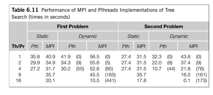
8- and 16-process results suggest that if a problem is large enough to warrant the use of many processes, the dynamic MPI program is much more scalable, and it can provide far superior performance. This is borne out by examination of a 17-city problem run with 16 processes: the dynamic MPI implementation has a run-time of 296 seconds, while the static implementation has a run-time of 601 seconds.

Note that times such as 0.1 second for the second problem running with 16 pro-cesses don’t really show superlinear speedup. Rather, the initial distribution of work has allowed one of the processes to find the best tour much faster than the initial distri-butions with fewer processes, and the dynamic partitioning has allowed the processes to do a much better job of load balancing.