Hashing Techniques That Allow Dynamic File Expansion

Hashing Techniques That Allow Dynamic File Expansion

A major drawback of the static hashing scheme just discussed is that the hash address space is fixed. Hence, it is difficult to expand or shrink the file dynamically. The schemes described in this section attempt to remedy this situation. The first scheme—extendible hashing—stores an access structure in addition to the file, and hence is somewhat similar to indexing (see Chapter 18). The main difference is that the access structure is based on the values that result after application of the hash function to the search field. In indexing, the access structure is based on the values of the search field itself. The second technique, called linear hashing, does not require additional access structures. Another scheme, called dynamic hashing, uses an access structure based on binary tree data structures..

These hashing schemes take advantage of the fact that the result of applying a hashing function is a nonnegative integer and hence can be represented as a binary number. The access structure is built on the binary representation of the hashing function result, which is a string of bits. We call this the hash value of a record. Records are distributed among buckets based on the values of the leading bits in their hash values.

Extendible Hashing. In extendible hashing, a type of directory—an array of 2^d bucket addresses—is maintained, where d is called the global depth of the directory. The integer value corresponding to the first (high-order) d bits of a hash value is used as an index to the array to determine a directory entry, and the address in that entry determines the bucket in which the corresponding records are stored. However, there does not have to be a distinct bucket for each of the 2^d directory locations. Several directory locations with the same first d bits for their hash values may contain the same bucket address if all the records that hash to these locations fit in a single bucket. 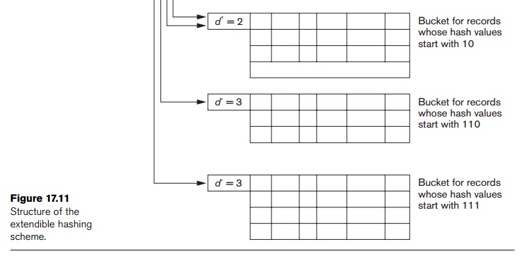A local depth d —stored with each bucket—specifies the number of bits on which the bucket contents are based. Figure 17.11 shows a directory with global depth d = 3.

The value of d can be increased or decreased by one at a time, thus doubling or halving the number of entries in the directory array. Doubling is needed if a bucket, whose local depth d is equal to the global depth d, overflows. Halving occurs if d > d for all the buckets after some deletions occur. Most record retrievals require two block accesses—one to the directory and the other to the bucket.

To illustrate bucket splitting, suppose that a new inserted record causes overflow in the bucket whose hash values start with 01—the third bucket in Figure 17.11. The records will be distributed between two buckets: the first contains all records whose hash values start with 010, and the second all those whose hash values start with 011. Now the two directory locations for 010 and 011 point to the two new distinct buckets. Before the split, they pointed to the same bucket. The local depth d of the two new buckets is 3, which is one more than the local depth of the old bucket.

If a bucket that overflows and is split used to have a local depth d equal to the global depth d of the directory, then the size of the directory must now be doubled so that we can use an extra bit to distinguish the two new buckets. For example, if the bucket for records whose hash values start with 111 in Figure 17.11 overflows, the two new buckets need a directory with global depth d = 4, because the two buckets are now labeled 1110 and 1111, and hence their local depths are both 4. The directory size is hence doubled, and each of the other original locations in the directory

is also split into two locations, both of which have the same pointer value as did the original location.

The main advantage of extendible hashing that makes it attractive is that the performance of the file does not degrade as the file grows, as opposed to static external hashing where collisions increase and the corresponding chaining effectively increases the average number of accesses per key. Additionally, no space is allocated in extendible hashing for future growth, but additional buckets can be allocated dynamically as needed. The space overhead for the directory table is negligible. The maximum directory size is 2^k, where k is the number of bits in the hash value. Another advantage is that splitting causes minor reorganization in most cases, since only the records in one bucket are redistributed to the two new buckets. The only time reorganization is more expensive is when the directory has to be doubled (or halved). A disadvantage is that the directory must be searched before accessing the buckets themselves, resulting in two block accesses instead of one in static hashing. This performance penalty is considered minor and thus the scheme is considered quite desirable for dynamic files.

Dynamic Hashing. A precursor to extendible hashing was dynamic hashing, in which the addresses of the buckets were either the n high-order bits or n − 1 high-order bits, depending on the total number of keys belonging to the respective bucket. The eventual storage of records in buckets for dynamic hashing is somewhat similar to extendible hashing. The major difference is in the organization of the directory. 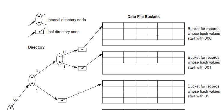Whereas extendible hashing uses the notion of global depth (high-order d bits) for the flat directory and then combines adjacent collapsible buckets into a bucket of local depth d − 1, dynamic hashing maintains a tree-structured directory with two types of nodes:

        Internal nodes that have two pointers—the left pointer corresponding to the 0 bit (in the hashed address) and a right pointer corresponding to the 1 bit.

        Leaf nodes—these hold a pointer to the actual bucket with records.

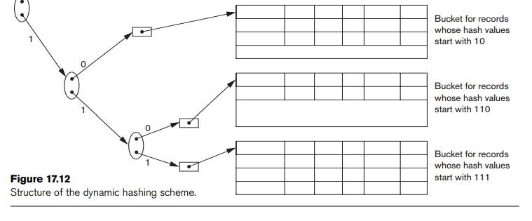
An example of the dynamic hashing appears in Figure 17.12. Four buckets are shown (“000”, “001”, “110”, and “111”) with high-order 3-bit addresses (corresponding to the global depth of 3), and two buckets (“01” and “10” ) are shown with high-order 2-bit addresses (corresponding to the local depth of 2). The latter two are the result of collapsing the “010” and “011” into “01” and collapsing “100” and “101” into “10”. Note that the directory nodes are used implicitly to determine the “global” and “local” depths of buckets in dynamic hashing. The search for a record given the hashed address involves traversing the directory tree, which leads to the bucket holding that record. It is left to the reader to develop algorithms for insertion, deletion, and searching of records for the dynamic hashing scheme.

Linear Hashing. The idea behind linear hashing is to allow a hash file to expand and shrink its number of buckets dynamically without needing a directory. Suppose that the file starts with M buckets numbered 0, 1, ..., M − 1 and uses the mod hash function h(K) = K mod M; this hash function is called the initial hash function h_i. Overflow because of collisions is still needed and can be handled by maintaining individual overflow chains for each bucket. However, when a collision leads to an overflow record in any file bucket, the first bucket in the file—bucket 0—is split into two buckets: the original bucket 0 and a new bucket M at the end of the file. The records originally in bucket 0 are distributed between the two buckets based on a different hashing function h_i+1(K) = K mod 2M. A key property of the two hash

functions h_i and h_i+1 is that any records that hashed to bucket 0 based on h_i will hash to either bucket 0 or bucket M based on h_i+1; this is necessary for linear hashing to work.

As further collisions lead to overflow records, additional buckets are split in the linear order 1, 2, 3, .... If enough overflows occur, all the original file buckets 0, 1, ..., M − 1 will have been split, so the file now has 2M instead of M buckets, and all buckets use the hash function h_i+1. Hence, the records in overflow are eventually redistributed into regular buckets, using the function h_i+1 via a delayed split of their buckets. There is no directory; only a value n—which is initially set to 0 and is incremented by 1 whenever a split occurs—is needed to determine which buckets have been split. To retrieve a record with hash key value K, first apply the function h_i to K; if h_i(K) < n, then apply the function h_i+1 on K because the bucket is already split. Initially, n = 0, indicating that the function h_i applies to all buckets; n grows linearly as buckets are split.

When n = M after being incremented, this signifies that all the original buckets have been split and the hash function h_i+1 applies to all records in the file. At this point, n is reset to 0 (zero), and any new collisions that cause overflow lead to the use of a new hashing function h_i+2(K) = K mod 4M. In general, a sequence of hashing func-tions h_i+j(K) = K mod (2^jM) is used, where j = 0, 1, 2, ...; a new hashing function h_i+j+1 is needed whenever all the buckets 0, 1, ..., (2^jM) − 1 have been split and n is reset to 0. The search for a record with hash key value K is given by Algorithm 17.3.

Splitting can be controlled by monitoring the file load factor instead of by splitting whenever an overflow occurs. In general, the file load factor l can be defined as l = r/(bfr _* N), where r is the current number of file records, bfr is the maximum number of records that can fit in a bucket, and N is the current number of file buckets. Buckets that have been split can also be recombined if the load factor of the file falls below a certain threshold. Blocks are combined linearly, and N is decremented appropriately. The file load can be used to trigger both splits and combinations; in this manner the file load can be kept within a desired range. Splits can be triggered when the load exceeds a certain threshold—say, 0.9—and combinations can be triggered when the load falls below another threshold—say, 0.7. The main advantages of linear hashing are that it maintains the load factor fairly constantly while the file grows and shrinks, and it does not require a directory.

Algorithm 17.3. The Search Procedure for Linear Hashing

if n = 0

then m ← h_j (K) (* m is the hash value of record with hash key K *) else begin

m ← h_j (K);

if m < n then m ← h_j+1 (K) end;

search the bucket whose hash value is m (and its overflow, if any);