Electromagnetic Theory - Introduction

ELECTROMAGNETIC THEORY

INTRODUCTION

Electromagnetic theory is a discipline concerned with the study of charges at rest and in motion. Electromagnetic principles are fundamental to the study of electrical engineering and physics. Electromagnetic theory is also indispensable to the understanding, analysis and design of various electrical, electromechanical and electronic systems. Some of the branches of study where

Electromagnetic principles find applications are:

1.        RF communication

2.        Microwave Engineering

3.        Antennas

4.        Electrical Machines

5.        Satellite Communication

6.        Atomic and nuclear research

7.        Radar Technology

8.        Remote sensing

9.        EMI EMC

10.   Quantum Electronics

11.   VLSI

Electromagnetic theory is a prerequisite for a wide spectrum of studies in the field of Electrical Sciences and Physics. Electromagnetic theory can be thought of as generalization of circuit theory. There are certain situations that can be handled exclusively in terms of field theory. In electromagnetic theory, the quantities involved can be categorized as source quantities and field quantities. Source of electromagnetic field is electric charges: either at rest or in motion. However an electromagnetic field may cause a redistribution of charges that in turn change the field and hence the separation of cause and effect is not always visible.

Sources of EMF:

·           Current carrying conductors.

·           Mobile phones.

·           Microwave oven.

·           Computer and Television screen.

·           High voltage Power lines.

Effects of Electromagnetic fields:

·           Plants and Animals.

·           Humans.

·           Electrical components.

Fields are classified as

·           Scalar field

·           Vector field.

Electric charge is a fundamental property of matter. Charge exist only in positive or negative integral multiple of electronic charge, -e, e= 1.60 × 10-19 coulombs. [It may be noted here that in 1962, Murray Gell-Mann hypothesized Quarks as the basic building blocks of matters. Quarks were predicted to carry a fraction of electronic charge and the existence of Quarks have been experimentally verified.] Principle of conservation of charge states that the total charge (algebraic sum of positive and negative charges) of an isolated system remains unchanged, though the charges may redistribute under the influence of electric field. Kirchhoff's Current Law (KCL) is an assertion of the conservative property of charges under the implicit assumption that there is no accumulation of charge at the junction.

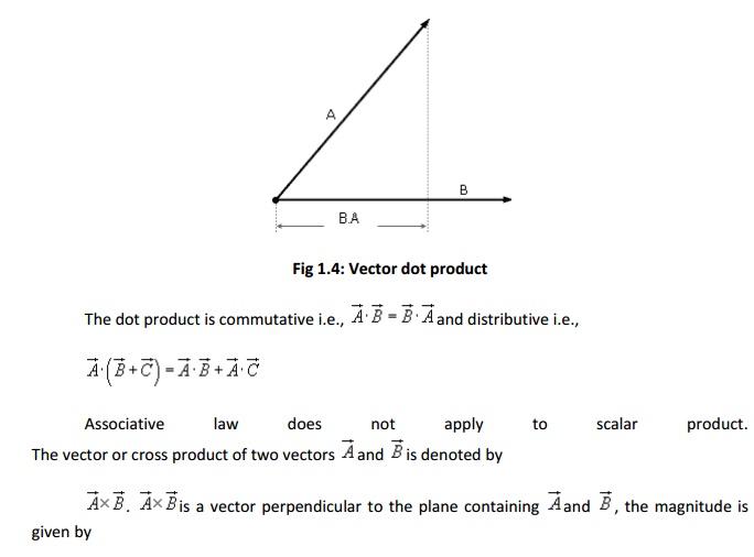
Electromagnetic theory deals directly with the electric and magnetic field vectors where as circuit theory deals with the voltages and currents. Voltages and currents are integrated effects of electric and magnetic fields respectively. Electromagnetic field problems involve three space variables along with the time variable and hence the solution tends to become correspondingly complex. Vector analysis is a mathematical tool with which electromagnetic concepts are more conveniently expressed and best comprehended. Since use of vector analysis in the study of electromagnetic field theory results in real economy of time and thought, we first introduce the concept of vector analysis.

Vector Analysis:

The quantities that we deal in electromagnetic theory may be either scalar or vectors [There are other class of physical quantities called Tensors: where magnitude and direction vary with co ordinate axes]. Scalars are quantities characterized by magnitude only and algebraic sign. A quantity that has direction as well as magnitude is called a vector. Both scalar and vector quantities are function of time and position . A field is a function that specifies a particular quantity everywhere in a region. Depending upon the nature of the quantity under consideration, the field may be a vector or a scalar field. Example of scalar field is the electric potential in a region while electric or magnetic fields at any point is the example of vector field.

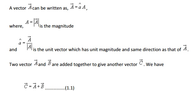
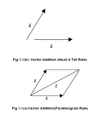
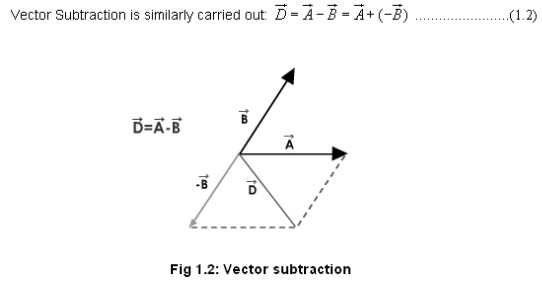
Let us see the animations in the next pages for the addition of two vectors, which has two rules:

1: Parallelogram law and  2: Head & tail rule

Co-ordinate Systems

In order to describe the spatial variations of the quantities, we require using appropriate co-ordinate system. A point or vector can be represented in a curvilinear coordinate system that may be orthogonal or non-orthogonal .

An orthogonal system is one in which the co-ordinates are mutually perpendicular. Non-orthogonal co-ordinate systems are also possible, but their usage is very limited in practice .

Let u = constant, v = constant and w = constant represent surfaces in a coordinate system, the surfaces may be curved surfaces in general. Furthur, let

be the unit vectors in the three coordinate directions(base vectors). In a general right handed orthogonal curvilinear systems, the vectors satisfy the following relations :

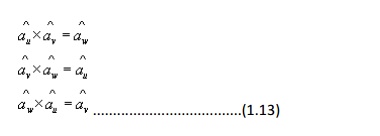
These equations are not independent and specification of one will automatically imply the other two. Furthermore, the following relations hold

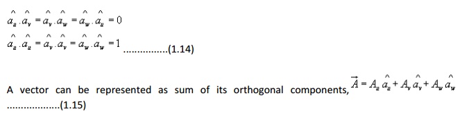
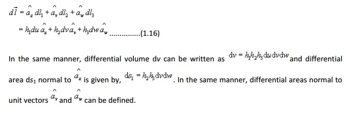
In general u, v and w may not represent length. We multiply u, v and w by conversion factors h1,h2 and h3 respectively to convert differential changes du, dv and dw to corresponding changes in length dl1, dl2, and dl3. Therefore

In the following sections we discuss three most commonly used orthogonal co-ordinate systems, viz:

1.        Cartesian (or rectangular) co-ordinate system

2.        Cylindrical co-ordinate system

3.        Spherical polar co-ordinate system

Cartesian Co-ordinate System :

In Cartesian co-ordinate system, we have, (u,v,w) = (x,y,z). A point P(x0, y0, z0) in Cartesian co-ordinate system is represented as intersection of three planes x = x0, y = y0 and z = z0. The unit vectors satisfies the following relation:

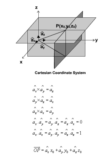
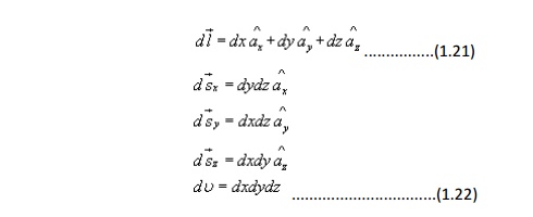
Since x, y and z all represent lengths, h1= h2= h3=1. The differential length, area and volume are defined respectively as

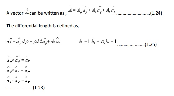
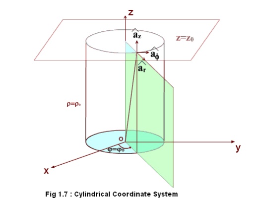
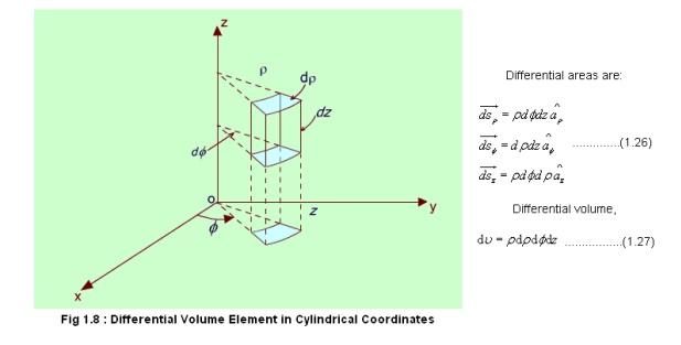
Cylindrical Co-ordinate System :

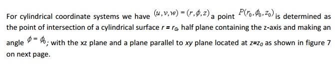
In cylindrical coordinate system, the unit vectors satisfy the following relations

Transformation between Cartesian and Cylindrical coordinates:

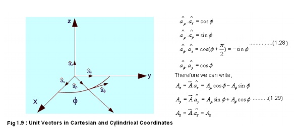
These relations can be put conveniently in the matrix form as:

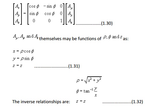
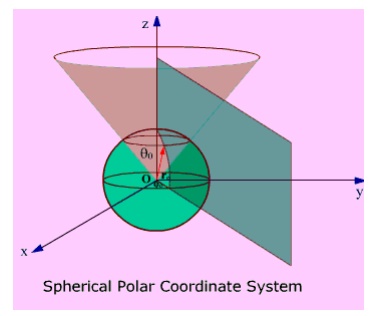
Fig 1.10: Spherical Polar Coordinate System

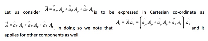
Thus we see that a vector in one coordinate system is transformed to another coordinate system through two-step process: Finding the component vectors and then variable transformation.

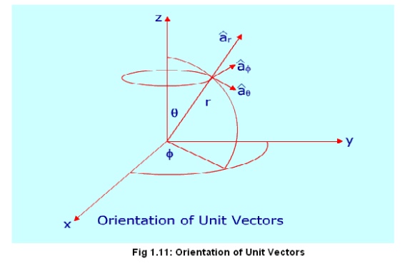
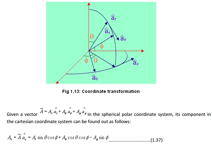
Spherical Polar Coordinates:

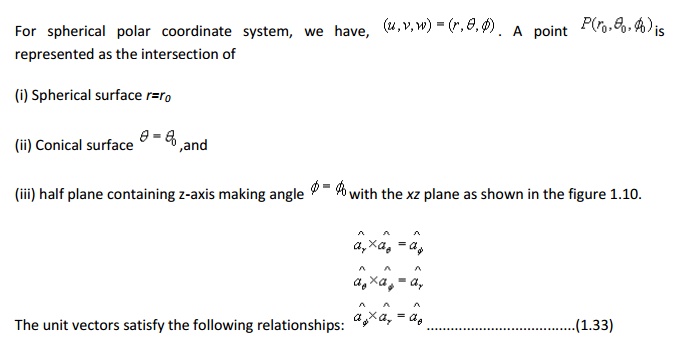
The orientation of the unit vectors are shown in the figure 1.11.

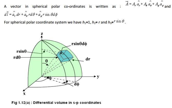
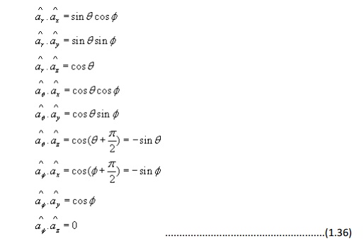
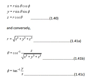
Coordinate transformation between rectangular and spherical polar:

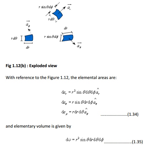
With reference to the Figure 1.12, the elemental areas are:

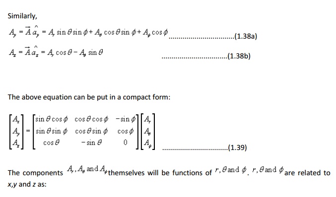
Using the variable transformation listed above, the vector components, which are functions of variables of one coordinate system, can be transformed to functions of variables of other coordinate system and a total transformation can be done.

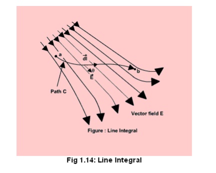
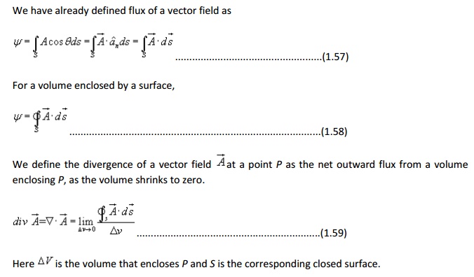
Line, surface and volume integrals

In electromagnetic theory, we come across integrals, which contain vector functions. Some representative integrals are listed below:

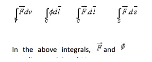
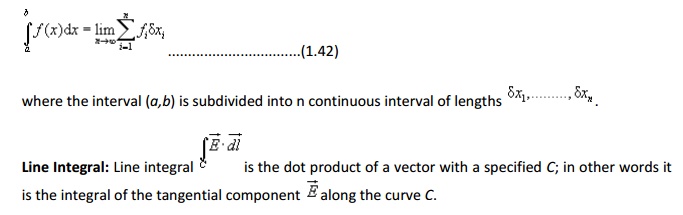
respectively represent vector and scalar function of space coordinates. C,S and V represent path, surface and volume of integration. All these integrals are evaluated using extension of the usual one-dimensional integral as the limit of a sum, i.e., if a function f(x) is defined over arrange a to b of values of x, then the integral is given by

Surface Integral :

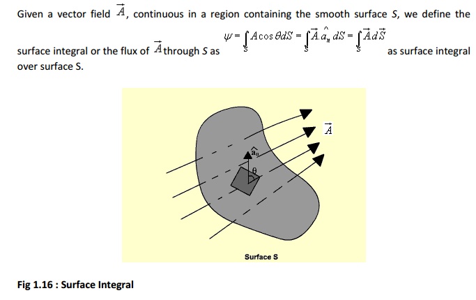
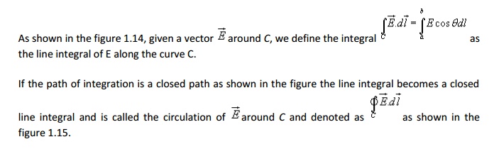
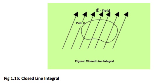
If the surface integral is carried out over a closed surface, then we write

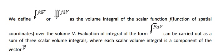
Volume Integrals:

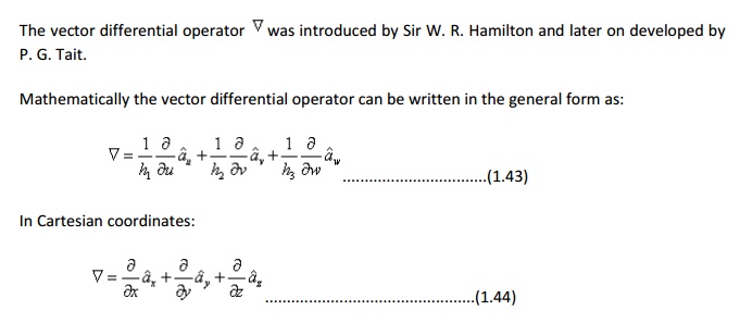
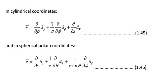
The Del Operator :

Gradient of a Scalar function:

Let us consider a scalar field V(u,v,w) , a function of space coordinates.

Gradient of the scalar field V is a vector that represents both the magnitude and direction of the maximum space rate of increase of this scalar field V.

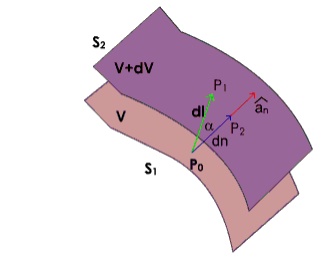
Fig 1.17 : Gradient of a scalar function

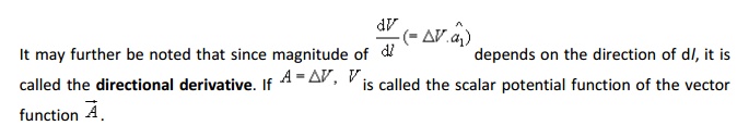
As shown in figure 1.17, let us consider two surfaces S1and S2 where the function V has constant magnitude and the magnitude differs by a small amount dV. Now as one moves from S1 to S2, the magnitude of spatial rate of change of V i.e. dV/dl depends on the direction of elementary path length dl, the maximum occurs when one traverses from S1to S2along a path normal to the surfaces as in this case the distance is minimum.

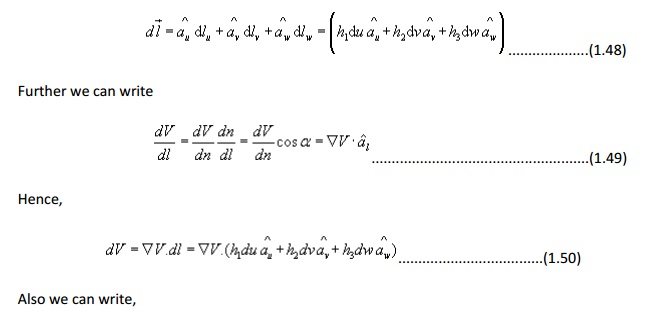
By our definition of gradient we can write:

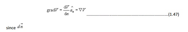
which represents the distance along the normal is the shortest distance between the two surfaces.

For a general curvilinear coordinate system

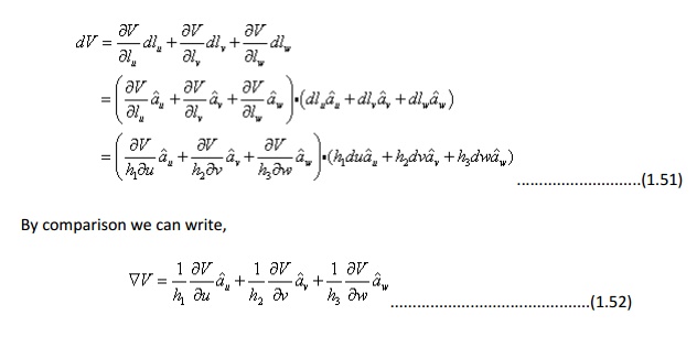
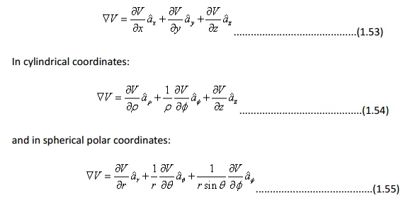
Hence for the Cartesian, cylindrical and spherical polar coordinate system, the expressions for gradient can be written as: In Cartesian coordinates:

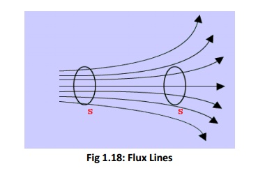
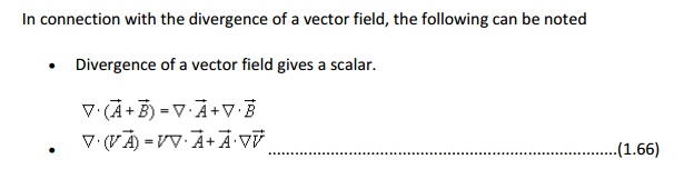
Divergence of a Vector Field:

In study of vector fields, directed line segments, also called flux lines or streamlines, represent field variations graphically. The intensity of the field is proportional to the density of lines. For example, the number of flux lines passing through a unit surface S normal to the vector measures the vector field strength.

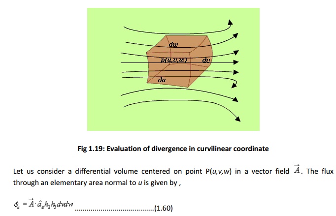
Net outward flux along u can be calculated considering the two elementary surfaces perpendicular to u .

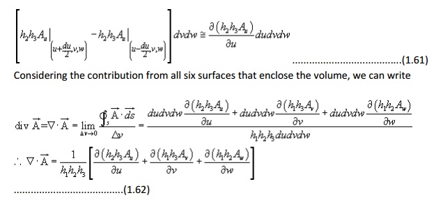
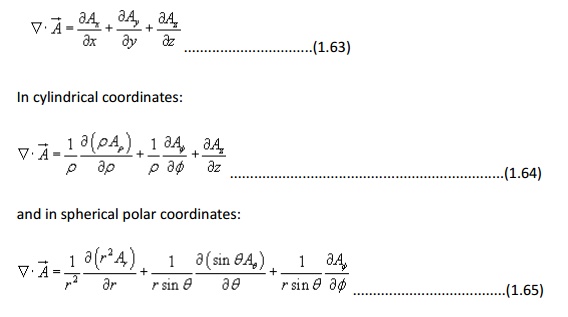
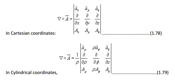
Hence for the Cartesian, cylindrical and spherical polar coordinate system, the expressions for divergence written

In Cartesian coordinates:

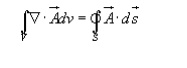
Divergence theorem :

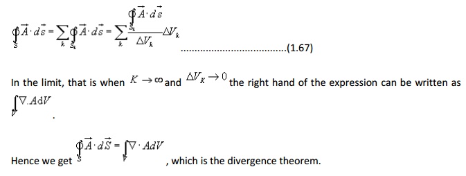
Divergence theorem states that the volume integral of the divergence of vector field is equal to the net outward flux of the vector through the closed surface that bounds the volume. Mathematically,

Proof:

Let us consider a volume V enclosed by a surface S . Let us subdivide the volume in large number of cells. Let the kth cell has a volume DV_k and the corresponding surface is denoted by Sk. Interior to the volume, cells have common surfaces. Outward flux through these common surfaces from one cell becomes the inward flux for the neighboring cells. Therefore when the total flux from these cells are considered, we actually get the net outward flux through the surface surrounding the volume. Hence we can write:

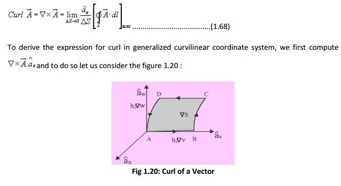
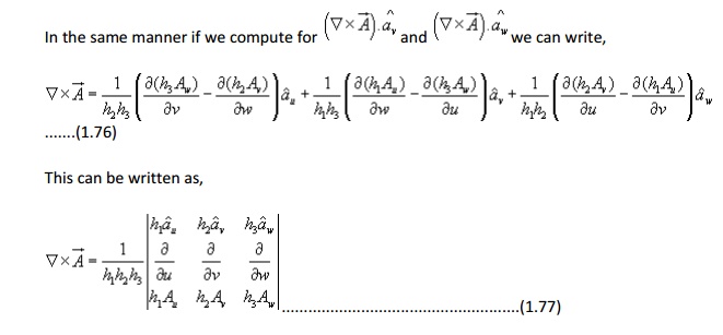
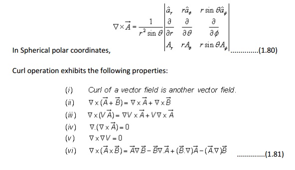
Curl of a vector field:

is defined as a vector whose magnitude is maximum of the net circulation per unit area when the area tends to zero and its direction is the normal direction to the area when the area is oriented in such a way so as to make the circulation maximum.

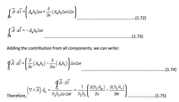
Therefore, we can write:

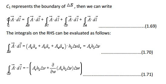
The negative sign is because of the fact that the direction of traversal reverses. Similarly,

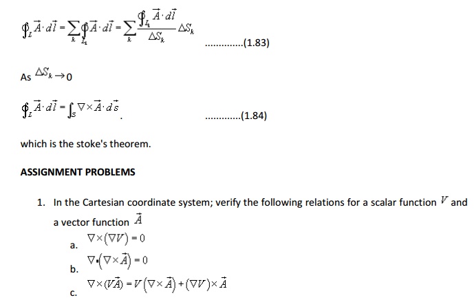
Stoke's theorem :

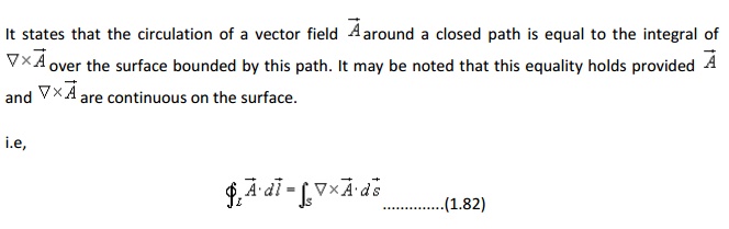
Proof: Let us consider an area S that is subdivided into large number of cells as shown in the figure 1.21.

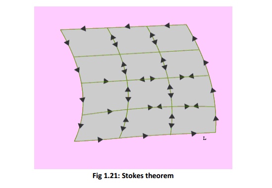
Let kth cell has surface area DSk and is bounded path Lk while the total area is bounded by path L. As seen from the figure that if we evaluate the sum of the line integrals around the elementary areas, there is cancellation along every interior path and we are left the line integral along path L. Therefore we can write,