Electrodynamic fields

Electrodynamic fields

Introduction:

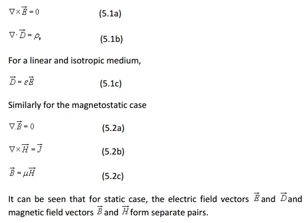
In our study of static fields so far, we have observed that static electric fields are produced by electric charges, static magnetic fields are produced by charges in motion or by steady current. Further, static electric field is a conservative field and has no curl, the static magnetic field is continuous and its divergence is zero. The fundamental relationships for static electric fields among the field quantities can be summarized as:

In this chapter we will consider the time varying scenario. In the time varying case we will observe that a changing magnetic field will produce a changing electric field and vice versa.

We begin our discussion with Faraday's Law of electromagnetic induction and then present the Maxwell's equations which form the foundation for the electromagnetic theory.

Faraday's Law of electromagnetic Induction

Michael Faraday, in 1831 discovered experimentally that a current was induced in a conducting loop when the magnetic flux linking the loop changed. In terms of fields, we can say that a time varying magnetic field produces an electromotive force (emf) which causes a current in a closed circuit. The quantitative relation between the induced emf (the voltage that arises from conductors moving in a magnetic field or from changing magnetic fields) and the rate of change of flux linkage developed based on experimental observation is known as Faraday's law. Mathematically, the induced emf can be written as

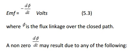
(a)     time changing flux linkage a stationary closed path.

(b)    relative motion between a steady flux a closed path.

(c)     a combination of the above two cases.

The negative sign in equation (5.3) was introduced by Lenz in order to comply with the polarity of the induced emf. The negative sign implies that the induced emf will cause a current flow in the closed loop in such a direction so as to oppose the change in the linking magnetic flux which produces it. (It may be noted that as far as the induced emf is concerned, the closed path forming a loop does not necessarily have to be conductive).

If the closed path is in the form of N tightly wound turns of a coil, the change in the magnetic flux linking the coil induces an emf in each turn of the coil and total emf is the sum of the induced emfs of the individual turns, i.e.,

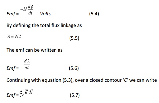
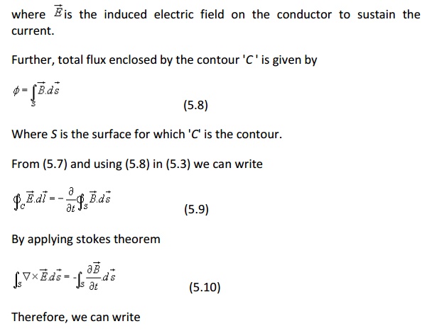
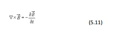
which is the Faraday's law in the point form

We have said that non zero dϕ/dt can be produced in a several ways. One particular case is when a time varying flux linking a stationary closed path induces an emf. The emf induced in a stationary closed path by a time varying magnetic field is called a transformer emf .

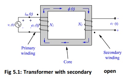
Example: Ideal transformer

As shown in figure 5.1, a transformer consists of two or more numbers of coils coupled magnetically through a common core. Let us consider an ideal transformer whose winding has zero resistance, the core having infinite permittivity and magnetic losses are zero.

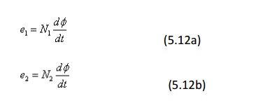
These assumptions ensure that the magnetization current under no load condition is vanishingly small and can be ignored. Further, all time varying flux produced by the primary winding will follow the magnetic path inside the core and link to the secondary coil without any leakage. If N₁ and N₂ are the number of turns in the primary and the secondary windings respectively, the induced emfs are

(The polarities are marked, hence negative sign is omitted. The induced emf is +ve at the dotted end of the winding.)

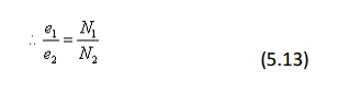
i.e., the ratio of the induced emfs in primary and secondary is equal to the ratio of their turns. Under ideal condition, the induced emf in either winding is equal to their voltage rating.

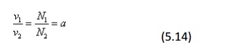
where 'a' is the transformation ratio. When the secondary winding is connected to a load, the current flows in the secondary, which produces a flux opposing the original flux. The net flux in the core decreases and induced emf will tend to decrease from the no load value. This causes the primary current to increase to nullify the decrease in the flux and induced emf. The current continues to increase till the flux in the core and the induced emfs are restored to the no load values. Thus the source supplies power to the primary winding and the secondary winding delivers the power to the load. Equating the powers

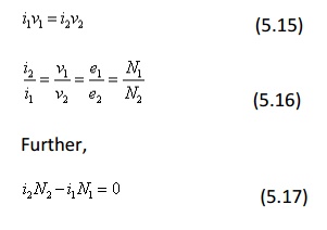
i.e., the net magnetomotive force (mmf) needed to excite the transformer is zero under ideal condition.

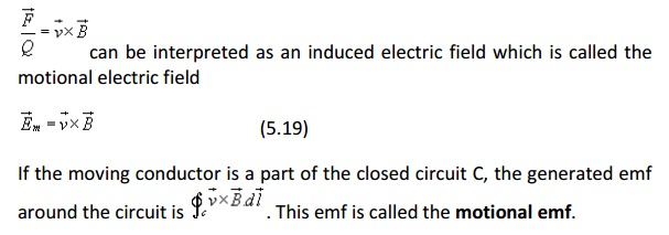
Motional EMF:

Let us consider a conductor moving in a steady magnetic field as shown in the fig 5.2.

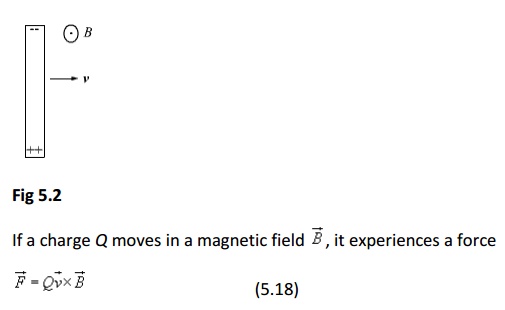
This force will cause the electrons in the conductor to drift towards one end and leave the other end positively charged, thus creating a field and charge separation continuous until electric and magnetic forces balance and an equilibrium is reached very quickly, the net force on the moving conductor is zero.

A classic example of motional emf is given in Additonal Solved Example No.1 .

Maxwell's Equation

Equation (5.1) and (5.2) gives the relationship among the field quantities in the static field. For time varying case, the relationship among the field vectors written as

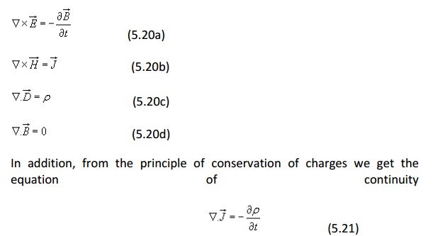
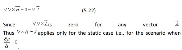
The equation 5.20 (a) - (d) must be consistent with equation (5.21). 

We observe that 

A classic example for this is given below . Suppose we are in the process of charging up a capacitor as shown in fig 5.3.

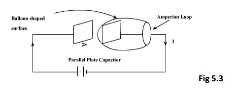
Let us apply the Ampere's Law for the Amperian loop shown in fig 5.3. I_enc = I is the total current passing through the loop. But if we draw a baloon shaped surface as in fig 5.3, no current passes through this surface and hence I_enc = 0. But for non steady currents such as this one, the concept of current enclosed by a loop is ill-defined since it depends on what surface you use. In fact Ampere's Law should also hold true for time varying case as well, then comes the idea of displacement current which will be introduced in the next few slides.

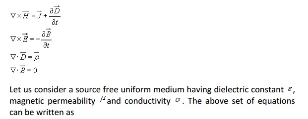
We can write for time varying case,

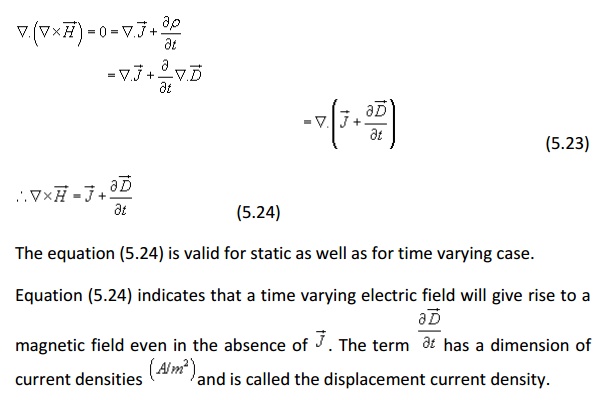
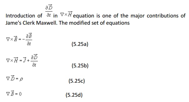
The modification of Ampere's law by Maxwell has led to the development of a unified electromagnetic field theory. By introducing the displacement current term, Maxwell could predict the propagation of EM waves. Existence of EM waves was later demonstrated by Hertz experimentally which led to the new era of radio communication.

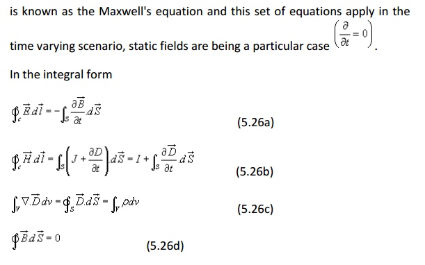
Boundary Conditions for Electromagnetic fields

The differential forms of Maxwell's equations are used to solve for the field vectors provided the field quantities are single valued, bounded and continuous. At the media boundaries, the field vectors are discontinuous and their behaviors across the boundaries are governed by boundary conditions. The integral equations(eqn 5.26) are assumed to hold for regions containing discontinuous media.Boundary conditions can be derived by applying the Maxwell's equations in the integral form to small regions at the interface of the two media. 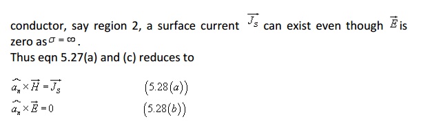The procedure is similar to those used for obtaining boundary conditions for static electric fields (chapter 2) and static magnetic fields (chapter 4). The boundary conditions are summarized as follows

With reference to fig 5.3

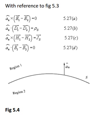
Equation 5.27 (a) says that tangential component of electric field is continuous across the interface while from 5.27 (c) we note that tangential  component of the magnetic field is discontinuous by an amount equal to  the surface current density. Similarly 5.27 (b) states that normal  component of electric flux density vector D(Bar) is discontinuous across the interface by an amount equal to the surface current density while normal  component of the magnetic flux density is continuous.  If one side of the interface, as shown in fig 5.4, is a perfect electric  

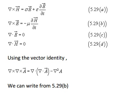
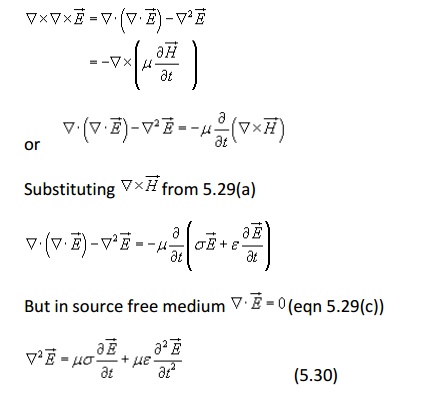
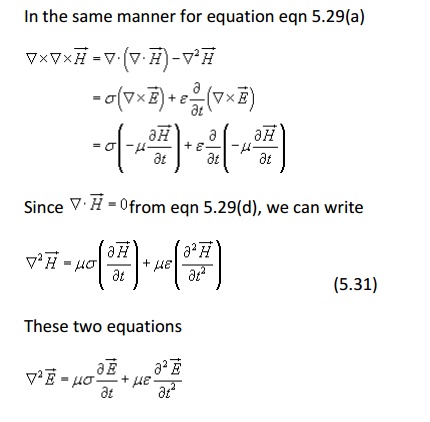
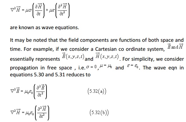
Wave equation and their solution: 

From equation 5.25 we can write the Maxwell's equations in the differential form as 

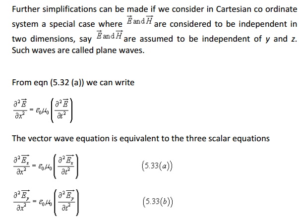
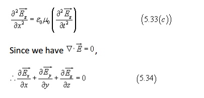
As we have assumed that the field components are independent of y and z eqn (5.34) reduces to

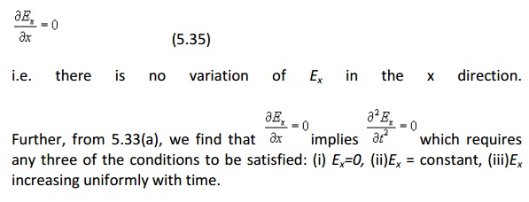
A field component satisfying either of the last two conditions (i.e (ii) and (iii))is not a part of a plane wave motion and hence E_x is taken to be equal to zero. Therefore, a uniform plane wave propagating in x direction does not have a field component (E or H) acting along x.

Without loss of generality let us now consider a plane wave having E_y component only (Identical results can be obtained for E_z component) .

The equation involving such wave propagation is given by

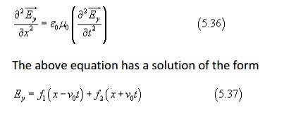
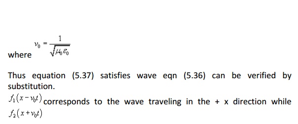
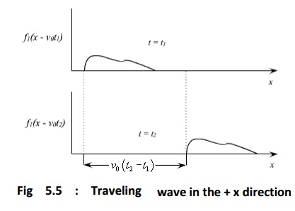
corresponds to a wave traveling in the -x direction. The general solution of the wave eqn thus consists of two waves, one traveling away from the source and other traveling back towards the source. In the absence of any reflection, the second form of the eqn (5.37) is zero and the solution can be written as

Such a wave motion is graphically shown in fig 5.5 at two instances of time t₁ and t₂.

Let us now consider the relationship between E and H components for the forward traveling wave.

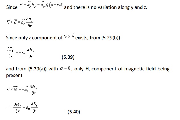
The constant of integration means that a field independent of x may also exist. However, this field will not be a part of the wave motion.

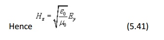
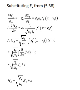
which relates the E and H components of the traveling wave.

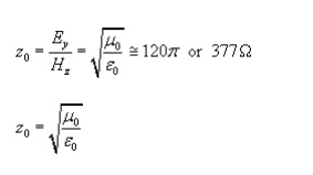
is called the characteristic or intrinsic impedance of the free space

ASSIGNMENT PROBLEMS