Effective Demand

Effective Demand

The starting point of Keynes theory of employment and income is the principle of effective demand. Effective demand denotes money actually spent by the people on products of industry. The money which entrepreneurs receive is paid in the form of rent, wages, interest and profit. Therefore effective demand equals national income.

An increase in the aggregate effective demand would increase the level of employment. A decline in total effective demand would lead to unemployment. Therefore, total employment of a country can be determined with the help of total demand of a country.

According to the Keynes theory of employment, “Effective demand signifies the money spent on consumption of goods and services and on investment. The total expenditure is equal to the national income, which is equivalent to the national output”. The relationship between employment and output of an economy depends upon the level of effective demand which is determined by the forces of aggregate supply and aggregate demand.

ED = Y = C + I = Output = Employment

Effective demand determines the level of employment in the economy. When effective demand increases, employment will increase. When effective demand decreases, the level employment will decline. The effective demand will be determined by two determinants namely consumption and investment expenditures. The consumption function depends upon income of the people and marginal propensity to consume. According to Keynes, if income increases, consumption will also increase but by less than the increase in income.

The rate of interest and marginal efficiency of capital determine the investment levels. Rate of interest depends on money supply and liquidity preference. Keynes has given importance to the concept of liquidity preference. Liquidity preference is based on three motives namely transaction motive, precautionary motive and speculative motive. MEC depends on two factors namely Prospective yield of capital asset and supply price of capital.

(For more details see Chapter 4)

1. Aggregate Demand Function (ADF)

In the Keynesian model, output is determined mainly by aggregate demand. The aggregate demand is the amount of money which entrepreneurs expect to get by selling the output produced by the number of labourers employed. Therefore, it is the expected income or revenue from the sale of output at different levels of employment.

Aggregate demand has the following four components:

1. Consumption demand

2. Investment demand

3. Government expenditure and

4. Net Export ( export – import )

The desired or planned demand (spending) is the amount that households, firms, the governments and the foreign purchasers would like to spend on domestic output. In other words, desired demand in the economy is the sum total of desired private consumption expenditure, desired investment expenditure, desired government spending and desired net exports (difference between exports and imports). Thus, the desired spending is called aggregate spending (demand), and can be expressed as:

AD = C + I + G + (X – M)

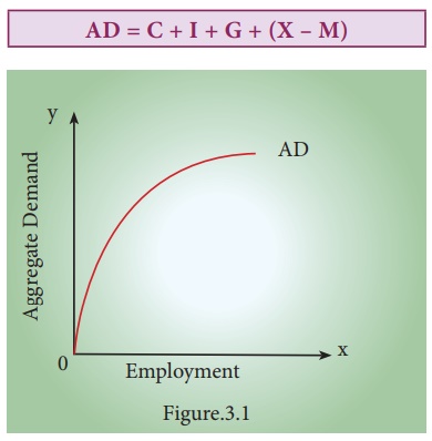
Figure 3.1. explains that aggregate demand price increases or decreases with an increase or decrease in the volume of employment. Aggregate demand curve increases at an increasing rate in the beginning and then increases at a decreasing rate. This shows that as income increases owing to increase in employment, expenditure of the economy increases at a decreasing rate.

2. Aggregate Supply Function (ASF)

Aggregate supply function is an increasing function of the level of employment. Aggregate supply refers to the value of total output of goods and services produced in an economy in a year. In other words, aggregate supply is equal to the value of national product, i.e., national income.

In other words, the aggregate supply refers to the required amount of labourers and materials to produce the necessary output. Employers hire labourers, purchase various inputs and raw materials to produce goods. Thus, production involves cost. If revenue from the sale of output produced exceeds the cost of production at a given level of employment and output, the entrepreneur would be encouraged to employ more labour and other inputs to produce more.

Aggregate supply price is the total amount of money that all entrepreneurs in an economy expect to receive from the sale of output produced by given number of labourers employed. The term ‘price’ refers to the amount of money received from the sale of output (sales proceeds). Hence, there are different aggregate prices for different levels of employment.

The components of aggregate supply are :

1. Aggregate (desired) consumption expenditure (C)

2. Aggregate (desired) private savings (S)

3. Net tax payments (T) (Total tax payment  to be received  by the government minus transfer payments, subsidy and interest payments to be incurred by the government) and

4. Personal (desired) transfer payments to the foreigners (Rf)(eg. Donations to international relief efforts)

Aggregate Supply = C + S + T + Rf = Aggregate income generated in the economy

The following figure 3.2 shows the shape of the two aggregate supply curves drawn for the assumption of fixed money wages and variable wages.

AGGREGATE SUPPLY CURVE

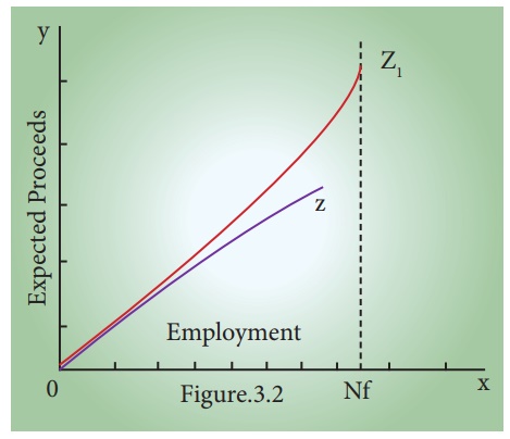
Z curve is linear where money wages remains fixed; Z₁ curve is non - linear since wage rate increases with employment. When full employment level of Nf is reached it is impossible to increase output by employing more men. So aggregate supply curve becomes inelastic (Vertical straight line).

The slope of the aggregate supply curve depends on the relation between the employment and productivity. The capital stock is often fixed and hence the law of diminishing marginal returns takes place as more workers are employed. Based upon this relation, the aggregate supply curve can be expected to slope upwards. In reality the aggregate supply curve will be like Z1 in figure 3.2. Therefore, the aggregate supply depends on the relationship between price and wages. If prices are high and wages low, the producers will try to employ labourers. If prices are low and wages high, investment will be curtailed, output will fall and there will be a reduction in the productive capacity. Thus aggregate supply is an important factor in determining the level of economic activity.

3. Equilibrium between ADF and ASF

Under the Keynes theory of employment, a simple two sector economy consisting of the household sector and the business sector is taken to understand the equilibrium between ADF and ASF. All the decisions concerning consumption expenditure are taken by the individual households, while the business firms take decisions concerning investment. It is also assumed that consumption function is linear and planned investment is autonomous.

There are two approaches to determination of the equilibrium level of income in Keynesian theory. These are :

1. Aggregate demand – Aggregate supply approach

2. Saving – Investment approach

In this chapter, out of these two, aggregate demand and aggregate supply approach is alone explained to understand the determination of equilibrium level of income and employment.

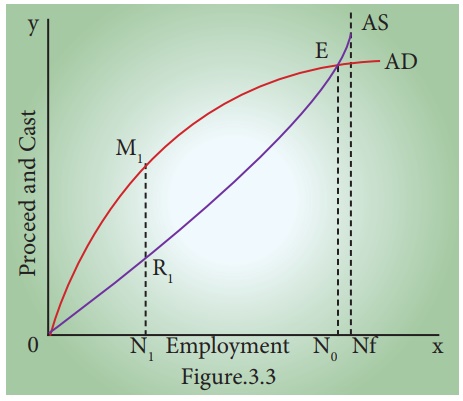
The concept of effective demand is more clearly shown in the figure 3.3

In the figure, the aggregate demand and aggregate supply reach equilibrium at point E. The employment level is N_o at that point.

At ON₁ employment, the aggregate supply is N ₁ R₁ . But they are able to produce M₁ N₁. The expected level of profit is M₁ R₁. To attain this level of profit, entrepreneurs will employ more labourers. The tendency to employ more labour will stop once they reach point E. At all levels of employment beyond, ON_o, the aggregate demand curve is below the aggregate supply curve indicating loss to the producers. Hence they will never employ more than ON_o labour. Thus effective demand concept becomes a crucial point in determining the equilibrium level of output in the capitalist economy or a free market economy in the Keynesian system.

It is important to note that the equilibrium level of employment need not be the full employment level (N₁) from the Figure 3.3, it is understood that the difference between N_o – N_f is the level of unemployment. Thus the concept of effective demand becomes significant in explaining the under employment equilibrium.