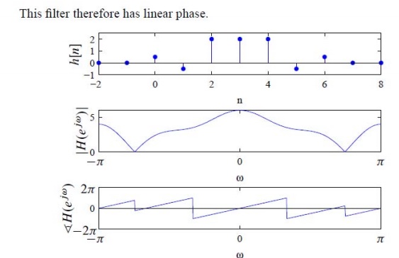
Chapter: Digital Signal Processing : FIR Filter Design
Digital Resonator
DIGITAL RESONATOR
A digital
resonator is a special two pole bandpass filter with a pair of complex
conjugate poles located near the unit circle. The name resonator refers to the
fact that the filter has a larger magnitude response in the vicinity of the
pole locations. Digital resonators are useful in many applications, including
simple bandpass filtering and speech generations.
IDEAL FILTERS ARE NOT PHYSICALLY REALIZABLE. Why?
Ideal
filters are not physically realizable because Ideal filters are anti-causal and
as only causal systems are physically realizable.
Proof:
Let take
example of ideal lowpass filter.
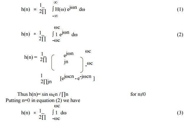
H(ω) = 1
for - ωc ≤ ω ≤ ωc
= 0 elsewhere
The unit
sample response of this ideal LPF can be obtained by taking IFT of H(ω).
LSI
system is causal if its unit sample response satisfies following condition.
h(n) = 0
for
n<0
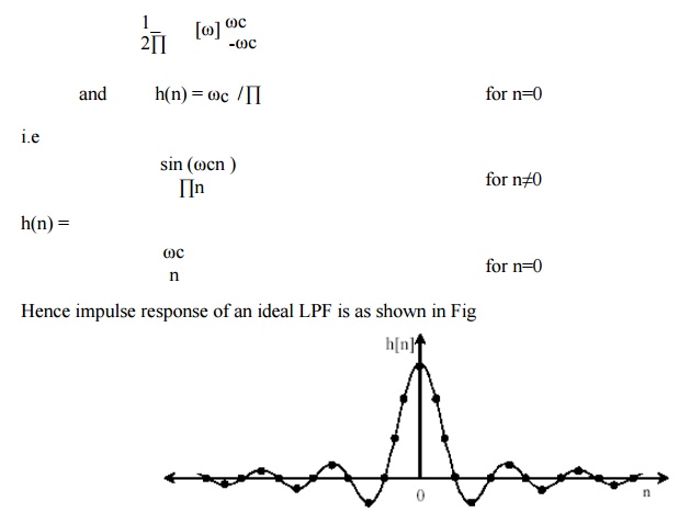
In above
figure h(n) extends -∞ to ∞ . Hence h(n) ≠0 for n<0. This means causality
condition is not satisfied by the ideal low pass filter. Hence ideal low pass
filter is non causal and it is not physically realizable.
EXAMPLES OF SIMPLE DIGITAL
FILTERS:
The
following examples illustrate the essential features of digital filters.
1. UNITY GAIN FILTER: yn
= xn
Each
output value yn is exactly the same as the corresponding input value
xn:
2. SIMPLE GAIN FILTER: yn
= Kxn (K = constant) Amplifier or attenuator) This simply applies a gain factor K to each input value:
3. PURE DELAY FILTER: yn
= xn-1
The
output value at time t = nh is simply
the input at time t = (n-1)h, i.e.
the signal is delayed by time h:
4. TWO-TERM DIFFERENCE FILTER: yn
= xn - xn-1
The
output is the average (arithmetic mean) of the current and previous input:
6. THREE-TERM AVERAGE FILTER: yn = (xn
+ xn-1 + xn-2) / 3
This is
similar to the previous example, with the average being taken of the current
and two previous inputs.
7. CENTRAL DIFFERENCE FILTER: yn
= (xn - xn-2) / 2
This is
similar in its effect to example (4). The output is equal to half the change in
the input signal over the previous two sampling intervals:
The order
of a digital filter can be defined as the number
of previous inputs (stored in the processor's memory) used to calculate the
current output.
This is
illustrated by the filters given as examples in the previous section.
Example (1): yn = xn
This is a
zero order filter, since the current
output yn depends only on the current
input xn and not on any previous
inputs.
Example (2): yn = Kxn
The order
of this filter is again zero, since
no previous outputs are required to give the current output value.
Example (3): yn = xn-1
This is a
first order filter, as one previous
input (xn-1) is required to calculate
y n. (Note that this filter is
classed as first-order because it uses one previous
input, even though the current input is not used).
Example (4): yn = xn - xn-1
This is
again a first order filter, since one
previous input value is required to give the current output.
Example (5): yn = (xn + xn-1)
/ 2
The order
of this filter is again equal to 1 since it uses just one previous input value.
Example (6): yn = (xn + xn-1
+ xn-2) / 3
To
compute the current output yn, two
previous inputs (xn-1 and xn-2) are needed; this is therefore a second-order filter.
Example (7): yn = (xn - xn-2)
/ 2
The
filter order is again 2, since the processor must store two previous inputs in
order to
compute the current output. This is unaffected by the absence of an explicit xn-1 term in the filter expression.
Q) For
each of the following filters, state the order of the filter and identify the
values of its coefficients:
(a) yn = 2xn - xn-1 A) Order = 1: a0 = 2, a1 = -1
(b) yn = xn-2 +
2xn-2 + xn-3 B) Order = 2: a0 = 0, a1 =
0, a2 = 1
(c) yn = xn - 2xn-1 C) Order = 3: a0 =
1, a1 = -2, a2 = 2, a3 = 1


Number
Representation
In digital signal processing, (B + 1)-bit
fixed-point numbers are usually represented as two’s- complement signed
fractions in the format
bo b-ib-2 …… b-B
The number represented is then
X = -bo + b-i2- 1 + b-22- 2
+ ••• + b-B 2-B (3.1)
where bo is the sign bit and the number range
is —1 <X < 1. The advantage of this representation is that the product of
two numbers in the range from — 1 to 1 is another number in the same range.
Floating-point numbers are represented as
X = (-1)s m2c (3.2)
where s is the sign bit, m is the mantissa, and
c is the characteristic or exponent. To make the representation of a number unique,
the mantissa is normalized so that 0.5 <m < 1.
Although floating-point numbers are always
represented in the form of (3.2), the way in which this representation is
actually stored in a machine may differ. Since m > 0.5, it is not necessary
to store the 2- 1 -weight bit of m, which is always set.
Therefore, in practice numbers are usually
stored as
X = (-1)s(0.5 + f)2c (3.3)
where f is an unsigned fraction, 0 <f <
0.5.
Most floating- point processors now use the
IEEE Standard 754 32-bit floating-point format for storing numbers. According
to this standard the exponent is stored as an unsigned integer p where
p = c + 126 (3.4)
Therefore,
a number is stored as
X = ( -1)s(0.5
+ f )2p - 1 2 6 (3.5) where s is the sign bit, f is a 23-b unsigned fraction in the range 0 <f < 0.5, and p is an 8 -b unsigned integer in the range 0 <p < 255. The total number of bits is
1 + 23 + 8 = 32. For example, in IEEE format 3/4 is written (-1)0 (0.5 + 0.25)2° so s = 0, p = 126, and f = 0.25.
The value X = 0 is a unique case and
is represented by all bits zero (i.e., s = 0, f = 0, and p = 0).
Although the 2-1-weight mantissa bit is not actually stored, it does
exist so the mantissa has 24 b plus a sign bit.
1. Fixed-Point Quantization
Errors
In fixed-
point arithmetic, a multiply doubles the number of significant bits. For
example, the product of the two 5-b numbers 0.0011 and 0.1001 is the 10 -b
number 00.000 110 11. The extra bit to the left of the decimal point can be
discarded without introducing any error. However, the least significant four of
the remaining bits must ultimately be discarded by some form of quantization so
that the result can be stored to 5 b for use in other calculations. In the
example above this results in 0.0010 (quantization by rounding) or 0.0001
(quantization by truncating). When a sum of products calculation is performed,
the quantization can be performed either after each multiply or after all
products have been summed with double-length precision.
We will
examine three types of fixed-point quantization—rounding, truncation, and
magnitude truncation. If X is an
exact value, then the rounded value will be denoted Qr (X), the
truncated value Qt (X), and the magnitude truncated value Qm t (X). If the quantized
value has B bits to the right of the decimal
point, the quantization step size is
A = 2-B
(3.6)
Since
rounding selects the quantized value nearest the unquantized value, it gives a
value which is never more than ± A /2 away from the exact value. If we denote
the rounding error by
fr = Qr(X) – X (3.7)
Truncation
simply discards the low-order bits, giving a quantized value that is always
less than or equal to the exact value so
- A < ft < 0 (3.9)
Magnitude
truncation chooses the nearest quantized value that has a magnitude less than
or equal to the exact value so
— A
<fmt <A (3.10)
The error resulting from quantization can be modeled as a random variable uniformly distributed over the appropriate error range. Therefore, calculations with roundoff error can be considered error-free calculations that have been corrupted by additive white noise.
2. Floating-Point Quantization
Errors
With
floating-point arithmetic it is necessary to quantize after both
multiplications and additions. The addition quantization arises because, prior
to addition, the mantissa of the smaller number in the sum is shifted right
until the exponent of both numbers is the same. In general, this gives a sum
mantissa that is too long and so must be quantized.
We will assume that quantization in floating-point arithmetic is performed by rounding. Because of the exponent in floating-point arithmetic, it is the relative error that is important.
Related Topics