Definition of the Transportation Model

DEFINITION OF THE TRANSPORTATION MODEL

The general problem is represented by the network in Figure 5.1. There are m sources and n destinations, each represented by a node. The arcs represent the routes linking the sources and the destinations. Arc (i, j) joining source i to destina-tion j carries two pieces of information: the transportation cost per unit, C_ij, and the amount shipped, Xij' The amount of supply at source i is ai and the amount of demand at destination j is b_j • The objective of the model is to determine the unknowns Xij  that will minimize the total transportation cost while satisfying all the supply and demand restrictions.

Example 5.1-1

MG Auto has three plants in Los Angeles, Detroit, and New Orleans, and two major distribution centers in Denver and Miami. The capacities of the three plants during the next quarter are 1000, 1500, and 1200 cars. The quarterly demands at the two distribution centers are 2300 and 1400 cars. The mileage chart between the plants and the distribution centers is given in Table 5.l.

The trucking company in charge of transporting the cars charges 8 cents per mile per car.

The transportation costs per car on the different routes, rounded to the closest dollar, are given in Table 5.2.

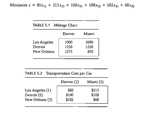
The LP model of the problem is given as

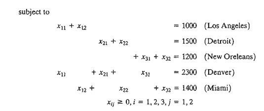
These constraints are all equations because the total supply from the three sources (= 1000 + 1500 + 1200 = 3700 cars) equals the total demand at the two destinations (= 2300 + 1400 = 3700 cars).

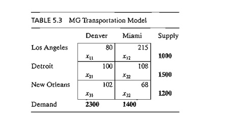
The LP model can be solved by the simplex method. However, with the special structure of the constraints we can solve the problem more conveniently using the transportation tableau shown in Table 5.3.

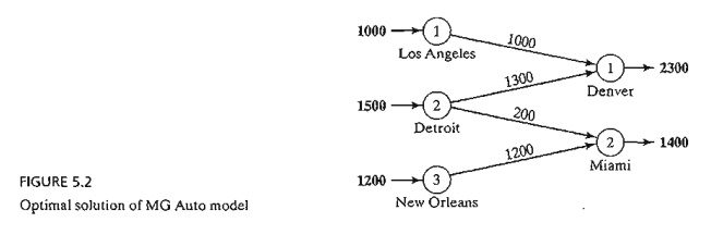
The optimal solution in Figure 5.2 (obtained by TORA) calls for shipping 1000 cars from Los Angeles to Denver, 1300 from Detroit to Denver, 200 from Detroit to Miami, and 1200 from New Orleans to Miami. The associated minimum transportation cost is computed as 1000 x $80 + 1300 x $100 + 200 x $108 + 1200 x $68 =  $313,200.

Balancing the Transportation Model. The transportation algorithm is based on the assumption that the model is balanced, meaning that the total demand equals the total supply. If the model is unbalanced, we can always add a dummy source or a dummy destination to restore balance.

Example 5.1-2

In the MG model, suppose that the Detroit plant capacity is 1300 cars (instead of 1500). The total supply (= 3500 cars) is less than the total demand (= 3700 cars), meaning that part of the demand at Denver and Miami will not be satisfied.

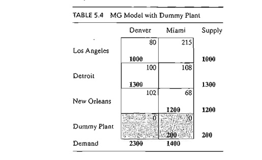
Because the demand exceeds the supply, a dummy source (plant) with a capacity of 200 cars (= 3700 - 3500) is added to balance the transportation model. The unit transportation costs from the dummy plant to the two destinations are zero because the plant does not exist.

Table 5.4 gives the balanced model together with its optimum solution. The solution shows that the dummy plant ships 200 cars to Miami, which means that Miami will be 200 cars short of satisfying its demand of 1400 cars.

We can make sure that a specific destination does not experience shortage by assigning a very high unit transportation cost from the dummy source to that destination. For example, a penalty of $1000 in the dummy-Miami cell will prevent shortage at Miami. Of course, we cannot use this "trick" with all the destinations, because shortage must occur somewhere in the system.

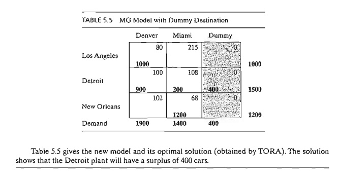
TIle case where the supply exceeds the demand can be demonstrated by assuming that the demand at Denver is 1900 cars only. In this case, we need to add a dummy distribution center to "receive" the surplus supply. Again, the unit transportation costs to the dummy distribution center are zero, unless we require a factory to "ship out" completely. In this case, we must assign a high unit transportation cost from the designated factory to the dummy destination.

PROBLEM SET 5.1A

1. True or False?

a.     To balance a transportation model, it may be necessary to add both a dummy source and a dummy destination.

b.     The amounts shipped to a dummy destination represent surplus at the shipping source.

c.      The amounts shipped from a dummy source represent shortages at the receiving destinations.

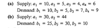
2. In each of the following cases, determine whether a dummy source or a dummy destination must be added to balance the model.

3. In Table 5.4 of Example 5.1-2, where a dummy plant is added, what does the solution mean when the dummy plant "ships" 150 cars to Denver and 50 cars to Miami?

*4. In Table 5.5 of Example 5.1-2, where a dummy destination is added, suppose that the De-troit plant must ship out all its production. How can this restriction be implemented in the model?

5. In Example 5.1-2, suppose that for the case where the demand exceeds the supply (Table 5.4), a penalty is levied at the rate of $200 and $300 for each undelivered car at Denver and Miami, respectively. Additionally, no deliveries are made from the Los Angeles plant to the Miami distribution center. Set up the model, and determine the optimal shipping schedule for the problem.

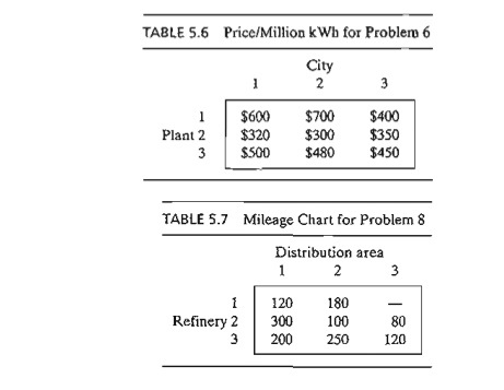
*6. Three electric power plants with capacities of 25, 40, and 30 million kWh supply electrici-ty to three cities. The maximum demands at the three cities are estimated at 30, 35, and 25 million kWh. The price per million kWh at the three cities is given in Table 5.6.

During the month of August, there is a 20% increase in demand at each of the three cities, which can be met by purchasing electricity from another network at a premium rate of $1000 per million kWh. The network is not linked to city 3, however. The utility company wishes to determine the most economical plan for the distribution and pur-chase of additional energy.

a. Formulate the problem as a transportation model.

b. Determine an optimal distribution plan for the utility company.

c. Determine the cost of the additional power purchased by each of the three cities.

7. Solve Problem 6, assuming that there is a 10% power transmission loss through the net-work.

8. Three refineries with daily capacities of 6, 5, and 8 million gallons, respectively, supply three distribution areas with daily demands of 4, 8, and 7 million gallons, respectively. Gasoline is transported to the three distribution areas through a network of pipelines.

The transportation cost is 10 cents per 1000 gallons per pipeline mile. Table 5.7 gives the mileage between the refineries and the distribution areas. Refinery 1 is not connected to distribution area 3.

a)     Construct the associated transportation model.

b)    Determine the optimum shipping schedule in the network.

*9. In Problem 8, suppose that the capacity of refinery 3 is 6 million gallons only and that distribution area 1 must receive all its demand. Additionally, any shortages at areas 2 and 3 will incur a penalty of 5 cents per gallon.

a)     Formula,te the problem as a transportation model.

b)    Determine the optimum shipping schedule.

10. In Problem 8, suppose that the daily demand at area 3 drops to 4 million gallons. Surplus production at refineries 1 and 2 is diverted to other distribution areas by truck. The trans-portation cost per 100 gallons is $1.50 from refinery 1 and $2.20 from refinery 2. Refinery 3 can divert its surplus production to other chemical processes within the plant.

Formulate the problem as a transportation model.

Determine the optimum shipping schedule.

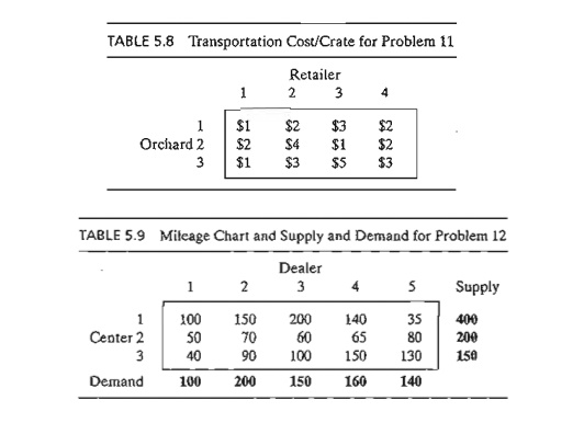
11. Three orchards supply crates of oranges to four retailers. The daily demand amounts at the four retailers are 150,150,400, and 100 crates, respectively. Supplies at the three orchards are dictated by available regular labor and are estimated at 150,200, and 250 crates daily. However, both orchards 1 and 2 have indicated that they could supply more crates, if necessary, by using overtime labor. Orchard 3 does not offer this option. The transportation costs per crate from the orchards to the retailers are given in Table 5.8.

a)                                Formulate the problem as a transportation model.

b)                               Solve the problem.

c)                                 How many crates should orchards 1 and 2 supply using overtime labor?

12. Cars are shipped from three distribution centers to five dealers. The shipping cost is based on the mileage between the sources and the destinations, and is independent of whether the truck makes the trip with partial or full loads. Table 5.9 summarizes the mileage between the distribution centers and the dealers together with the monthly sup-ply and demand figures given in number of cars. A full truckload includes 18 cars. The transportation cost per truck mile is $25.

a)     Fonnulate the associated transportation model.

b)    Determine the optimal shipping schedule.

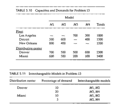
13. MG Auto, of Example 5.1-1, produces four car models: MI, M2, M3, and M4. The Detroit. plant produces models Ml, M2, and M4. Models MI and M2 are also produced in New Orleans. The Los Angeles plant manufactures models M3 and M4. The capacities of the various plants and the demands at the distribution centers are given in Table 5.10.

The mileage chart is the same as given in Example 5.1-1, and the transportation rate remains at 8 cents per car mile for all models. Additionally, it is possible to satisfy a per-centage of the demand for some models from the supply of others according to the speci-fications in Table 5.11.

a)     Formulate the corresponding transportation model.

b)   Determine the optimum shipping schedule.

(Hint: Add four new destinations corresponding to the new combinations [MI, M2], [M3, M4], [Ml, M2], and [M2, M4]. The demands at the new destinations are determined from the given percentages.)