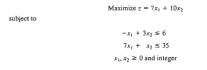
Chapter: Operations Research: An Introduction : Integer Linear Programming
Cutting-Plane Algorithm
Cutting-Plane Algorithm
As in the
B&B algorithm, the cutting-plane algorithm also starts at the continuous
optimum LP solution. Special constraints (called cuts) are added to the solution space in a manner that renders an
integer optimum extreme point. In Example 9.2-2, we first demonstrate
graphically how cuts are used to produce an integer solution and then implement
the idea algebraically.
Example 9.2-2
Consider the following ILl'.
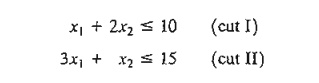
The cutting-plane algorithm modifies the solution space by adding cuts that produce an optimum integer extreme point. Figure 9.10 gives an example of two such cuts.
Initially,
we start with the continuous LP optimum z
= 66(1/2), x1 = 4(1/2), x2 = 3(4/7). Next, we
add cut I, which produces the (continuous) LP optimum solution z = 62, x1 = 4(4/7), x2 = 3. Then, we add cut II, which,
together with cut I and the original constraints, produces the LP optimum z =
58, xl =
4, x2 = 3. The last solution is all integer, as
desired.
The added
cuts do not eliminate any of the original feasible integer points, but must
pass through at least one feasible or infeasible integer point. These are basic
requirements of any cut.
FIGURE 9.10
Illustration of the use of cuts in ILP
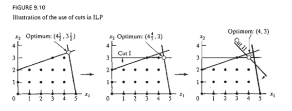
It is purely accidental that a
2-variable problem used exactly 2 cuts to reach the optimum integer solution.
In general, the number of cuts, though finite, is independent of the size of
the problem, in the sense that a problem with a small number of variables and
constraints may re-quire more cuts than a larger problem.
Next, we
use the same example to show how the cuts are constructed and implemented
algebraically.
Given the
slacks x3 and x4 for constraints 1 and 2, the optimum LP tableau is given as
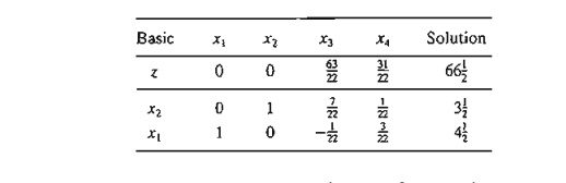
The
optimum continuous solution is z = 66(1/2), x1= 4(1/2), x2 = 3(1/2), x3 = 0, x4 = 0. The cut is developed under
the assumption that all the variables
(including the slacks x3
and x4) are integer. Note
also that because all the original objective coefficients are integer in this
example, the value of z is integer as
well.
The
information in the optimum tableau can be written explicitly as
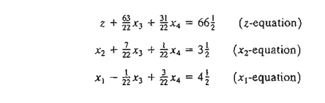
A
constraint equation can be used as a source row for generating a cut, provided
its right-hand side is fractional. We also note that the z-equation can be used
as a source row because z happens to
be integer in this example. We will demonstrate how a cut is generated from
each of these source rows, starting with the z-equation.
First, we
factor out all the noninteger coefficients of the equation into an integer
value and a fractional component, provided
that the resulting fractional component is strictly positive. For example,
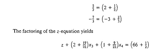
Moving
all the integer components to the left-hand side and all the fractional
components to the right-hand side, we get
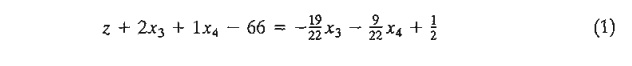
Because x3 and x4 are nonnegative and all fractions are originally
strictly positive, the right-hand side must satisfy the following inequality:
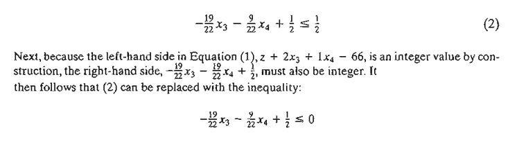
This
result is justified because an integer value ≤ 1/2 must necessarily be ≤ 0 .
The last
inequality is the desired cut and it represents a necessary (but not sufficient) condition for obtaining an integer
solution. It is also referred to as the fractional
cut because all its co-efficients are fractions.
Because x3 = x4 = 0 in the optimum continuous LP tableau given above,
the current continu-ous solution violates the cut (because it yields 1/2 ≤ 0). Thus, if we add this cut
to the optimum tableau, the resulting optimum extreme point moves the solution
toward satisfying the integer requirements.
Before
showing how a cut is implemented in the optimal tableau, we will demonstrate
how cuts can also be constructed from the constraint equations. Consider the x1-row:
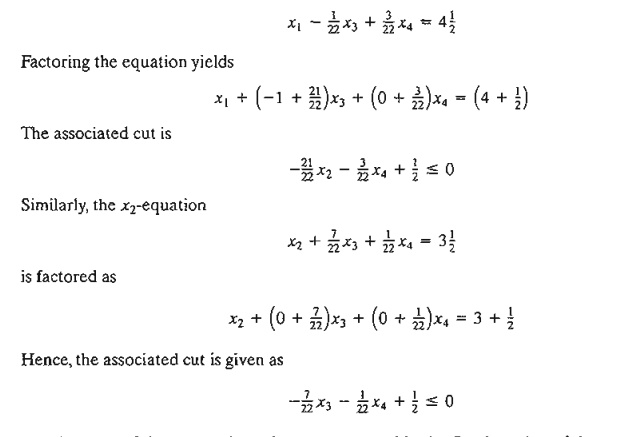
Anyone of
three cuts given above can be used in the first iteration of the cutting-plane
a1gorithm. It is not
necessary to generate all three cuts before selecting one.
Arbitrarily
selecting the cut generated from the x2-row,
we can write it in equation form as
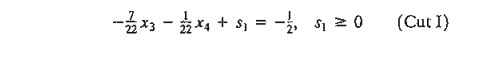
This
constraint is added to the LP
optimum tableau as follows:
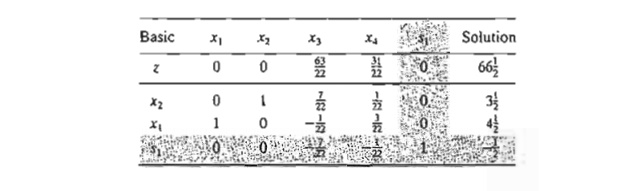
The
tableau is optimal but infeasible. We apply the dual simplex method (Section
4.4.1) to recover feasibility, which yields
The last
solution is still noninteger in xl and x3. Let us arbitrarily select xl
as the next source row-that is,
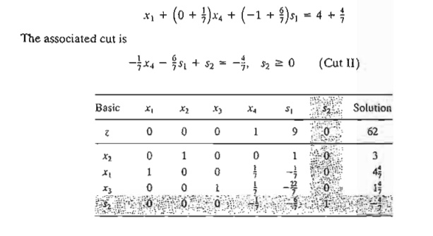
The dual
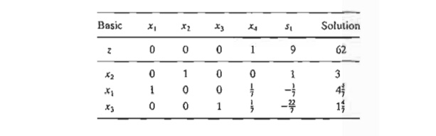
simplex method yields the following tableau:
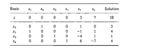
The
optimum solution (xl = 4, x2 = 3, z = 58) is all integer. It is not
accidental that all the coefficients of the last tableau are integers, a
property of the implementation of the fractional cut.
Remarks. It is
important to point out that the fractional cut assumes that all the variables, including slack and surplus, are integer. This means that the cut
deals with pure integer problems only. The importance of this assumption is
illustrated by an example.
Consider
the constraint
From the
standpoint of solving the associated ILP, the constraint is treated as an
equation by using the nonnegative slack sl-that is,
The
application of the fractional cut assumes that the constraint has a feasible
integer solution in all xl, x2, and sl. However, the
equation above will have a feasible integer solution in xl and x2 only if
x1 is noninteger. This means that the cutting-plane algorithm will show
that the problem has no feasible integer solution, even though the variables of
concern, xl and x2, can assume feasible integer
values.
There are
two ways to remedy this situation.
1. Multiply
the entire constraint by a proper constant to remove all the fractions. For
example, multiplying the constraint above by 6, we
get
Any
integer solution of x1 and x2 automatically yields integer
slack. However, this type of conversion is appropriate for only simple
constraints, because the magnitudes of the integer coefficients may become
excessively large in some
cases.
2. Use a
special cut, called the mixed cut, which allows only a subset of variables to
assume integer values, with all the other variables (including slack and
surplus) remaining continuous. The details of this cut will not be presented in
this chapter (see Taha, 1975, pp. 198-202).
PROBLEM SET 9.2B
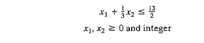
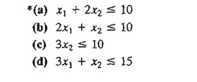
1. In Example 9.2-2, show graphically whether or not each of the following
constraints can form a legitimate cut:
2. In Example 9.2-2, show graphically how the following two (legitimate)
cuts can lead to the optimum integer solution:
3. Express
cuts I and II of Example 9.2-2 in terms of Xl and X2 and show
that they are the same ones used graphically in Figure 9.10.
4. In Example 9.2-2, derive cut II from the x3-row. Use the new cut to
complete the solution of the example.
5. Show
that, even though the following problem has a feasible integer solution in x1 and x2, the fractional cut would not yield a feasible solution unless all the
fractions in the con-straint were eliminated.
6. Solve the following problems by the fractional cut, and compare the
true optimum integer solution with the solution obtained by rounding the
continuous optimum.
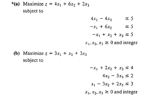
*(a) Maximize z = 4XI + 6X2 + 2X3 subject to
Related Topics