Chapter: Multicore Application Programming For Windows, Linux, and Oracle Solaris : Scaling with Multicore Processors
Constraints to Application Scaling
Constraints
to Application Scaling
Most applications, when run in parallel over multiple cores, will get
less than linear speedup. We discussed this in Chapter 3, “Identifying
Opportunities for Parallelism.” Amdahl’s law indicates that a section of serial
code will limit the scalability of the appli-cation over multiple cores. If the
application spends half of its runtime in a section of code that has been made
parallel and half in a section of code that has not, then the best that can be
achieved with two threads is that the application will run in three-quarters of
the original time. The best that could ever be achieved would be for the code
to run in about half the original time, given enough threads.
However, there will be other limitations that stop an application from
scaling per-fectly. These limitations could be hardware bottlenecks where some
part of the system has reached a maximum capacity. Adding more threads divides
this total amount of resources between more consumers but does not increase the
amount available. Scaling can also be limited by hardware interactions where
the presence of multiple threads causes the hardware to become less effective.
Software limitations can also constrain scal-ing where synchronization
overheads become a significant part of the runtime.
Performance
Limited by Serial Code
As previously discussed, the serial sections of code will limit how fast
an application can execute given unlimited numbers of threads. Consider the
code shown in Listing 9.1. This application has two sections of code; one
section is serial code, and the other sec-tion is parallel code.
Listing 9.1 Application
with Serial and Parallel Sections
#include <math.h> #include <stdlib.h>
void func1( double*array, int n )
{
for( int i=1; i<n; i++ )
{
array[i] += array[i-1];
}
}
void func2( double *array,int n )
{
#pragma omp parallel for for( int i=0; i<n; i++
)
{
array[i] = sin(array[i]);
}
}
int main()
{
double * array = calloc( sizeof(double), 1024*1024 ); for ( int i=0;
i<100; i++ )
{
func1( array, 1024*1024 ); func2( array, 1024*1024
);
}
return 0;
}
Listing 9.2 shows the profile from the application when it is
parallelized using OpenMP and run with a single thread. The application runs
for nearly 16 seconds; this is the wall time. The user time is the time spent
by all threads executing user code. More than half of the wall time is spent in
the sin()
function, about five seconds is spent in func2(), and about two seconds is spent in func1(). So, 14 of the 16 seconds of run-time are spent in code that can be
executed in parallel.
Listing 9.2 Profile
of Code Run with a Single Thread
Excl. Excl. Name
User CPU Wall
sec. sec.
15.431 15.701 <Total>
8.616 8.756 sin
4.963 5.034 func2
1.821 1.831 func1
0.020 0.030 memset
0.010 0.010 <OMP-overhead>
If two threads were to run this application, we
would expect each thread to take about seven seconds to complete the parallel
code and one thread to spend about two seconds completing the serial code. The
total wall time for the application should be about nine seconds. The actual
profile, when run with two threads, can be seen in Listing 9.3.
Listing 9.3 Profile
of Code Run with Two Threads
Excl. Excl. Name
User
CPU Wall
sec. sec.
15.421 8.956 <Total>
8.526 4.413 sin
4.973 2.432 func2
1.831 1.851 func1
0.030 0.030 memset
0.030 0.140 <OMP-implicit_barrier>
0.030 0.040 <OMP-overhead>
The first thing that is important to notice is that
the total amount of user time remained the same. This is the anticipated
result; the same amount of work is being per-formed, so the time taken to
complete it should remain the same.
The second observation is that the wall time
reduces to about nine seconds. This is the amount of time that we calculated it
would take.
The third observation is that the synthetic
routines <OMP-implicit_barrier> and <OMP-overhead> accumulate
a small amount of time. These represent the costs of the
OpenMP implementation. The time attributed to the
routines is very small, so they are not a cause for concern.
For a sufficiently large number of threads, we would hope that the
runtime for the code could get reduced down to the time it takes for the serial
region to complete, plus a small amount of time for the parallel code and any
necessary synchronization. Listing 9.4 shows the same code run with 32 threads.
Listing 9.4 Profile of Code Run with 32 Threads
Excl. Excl. Name User CPU Wall
sec.sec.
17.1623.192 <Total>
9.5270.410 sin
5.5940.190 func2
1.9111.991 func1
0.0900.520 <OMP-implicit_barrier>
0.0300.040 memset
0.0100.<OMP-idle>
With perfect scaling, we would expect the runtime
of the application with 32 threads to be 2 seconds of serial time plus 14 seconds
divided by 32 threads, making a total of just under 3 seconds. The actual wall
time is not that far from this ideal number. However, notice that the total
user time has increased.
This code is actually running on a single multicore
processor, so the increase in user time probably indicates that the processor
is hitting some scaling limits at this degree of utilization. The rest of the
chapter will discuss what those limits could be.
The other thing to observe is that although the
user time has increased by two sec-onds, this increase does not have a
significant impact on the total wall time. This should not be a surprising
result. A 2-second increase in user time spread over 32 threads repre-sents a
1/16th of a second increase in per thread, which is unlikely to be noticeable
in the elapsed time, or wall time, of the application’s run.
This code has scaled very well. There remains two
seconds of serial time and no amount of threads will reduce that, but the time
for the parallel region has scaled very well as the number of threads has
increased.
Superlinear
Scaling
Imagine that you hurt your hand and were no long able to use both hands
to type but you still had a report to finish. For most people, it would take
more than twice as long to produce the report using one hand as using two. When
your hand recovers, the rate at which you can type will more than double. This
is an example of superlinear speedup.
You double the resources yet get more than double the performance as a result.
It’s easy to explain for this particular situation. With two hands, all the
keys on the keyboard are within easy reach, but with only one hand, it is not
possible to reach all the keys without having to move your hand.
In most instances, going from one thread to two will result in, at most,
a doubling of performance. However, there will be applications that do see
superlinear scaling—the application ends up running more than twice as fast.
This is typically because the data that the application uses becomes cache
resident at some point. Imagine an application that uses 4MB of data. On a
processor with a 2MB cache, only half the data will be resident in the cache.
Adding a second processor adds an additional 2MB of cache; then all the data
becomes cache resident, and the time spent waiting on memory becomes
sub-stantially lower.
Listing 9.5 shows a modification of the program in
Listing 9.1 that uses 64MB of memory.
Listing 9.5 Program
with 64MB Memory Footprint
#include
<stdlib.h>
double
func1( double*array, int n )
{
double total = 0.0;
#pragma omp parallel for reduction(+:total) for(
int i=1; i<n; i++ )
{
total += array[i^29450];
}
return total;
}
int
main()
{
double * array = calloc( sizeof(double), 8192*1024 ); for( int i=0; i<100; i++ )
{
func1( array, 8192*1024 );
}
}
When the program is run on a single processor with
32MB of second-level cache, the program takes about 25 seconds to complete.
When run using two threads on the same processor, the code completes in about
12 seconds and takes 25 seconds of user time. This is the anticipated
performance gain from using multiple threads. The code takes half the time but
does the same amount of work. However, when run using two threads, with each
thread bound to a separate processor, the program runs in just over four
sec-onds of wall time, taking only eight seconds of user time.
Adding the second processor has increased the
amount of cache available to the pro-gram, causing it to become cache resident.
The data in cache has a lower access latency, so the program runs significantly
faster.
It is a different situation on a multicore processor. Adding an
additional thread, partic-ularly if it resides on the same core, does not
substantially increase the amount of cache available to the program. So, a
multicore processor is unlikely to see superlinear speedup.
Workload
Imbalance
Another common software issue is workload
imbalance, when the work is not evenly dis-tributed over the threads. We
have already seen an example of this in the Mandelbrot
example in Chapter 7. The code in
Listing 9.6 has a very deliberate workload imbalance. The number of iterations in the compute() function is proportional to the square of the value passed into it; the
larger the number passed into the function, the more time it will take to
complete.
A parallel loop iterates over a range from small values up to large
values, passing each value into the function. If the work is statically
distributed, the threads that get the initial iterations will spend less time
computing the result than the threads that get the later iterations.
Listing 9.6 Code
Exhibiting Workload Imbalance
#include <stdlib.h>
int compute( int value )
{
value = value*value; while ( value > 0 )
{
value = value - 12.0;
}
return value;
}
int main()
{
#pragma omp parallel for for( int i=0; i<3000;
i++ )
{
compute( i );
}
}
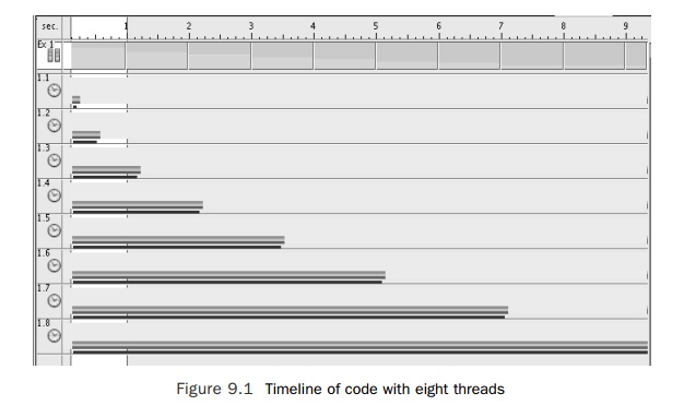
Figure 9.1 shows the timeline view of running the code with eight
threads. Each horizontal bar represents a thread actively running user code.
The duration of the run is governed by the time taken by the longest thread.
The longest threads completed in just over nine seconds. In those 9 seconds,
the eight threads accumulated 27 seconds of user time. The user time represents
the amount of work that the threads actually completed. If those 27 seconds of
user time had been spread evenly across the eight threads, then the application
would have completed in about 3.5 seconds.
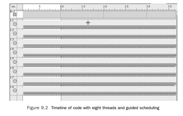
Changing the scheduling of the parallel loop to guided scheduling results in the time-line shown in Figure 9.2. After this change, the work is evenly distributed across the threads, and the application runs in just over 3.5 seconds.
Hot Locks
Contended (or hot) mutex locks are one of the common causes of poor application
scal-ing. This comes about when there are too many threads contending for a
single resource protected by a mutex. There are two attributes of the program
conspiring to produce the hot lock.
n The first attribute is the number of threads needed to lock a single
mutex. This is the usual reason for poor scaling; there are just too many
threads trying to access this one resource.
n The second, more subtle, issue is that the interval between a single
thread’s accesses of the resource is too short. For example, imagine that each
thread in an applica-tion needs to access a resource for one second and then
does not access that resource again for nine seconds. In those nine seconds,
another nine threads could access the resource without a conflict. The
application would be able to scale very well to ten threads, but if an eleventh
thread was added, the application would not scale as well, since this
additional thread would delay the other threads from access to the resource.
These two factors result in the more complex
behavior of an application with multi-ple threads. The application may scale to
a particular number of threads but start scaling poorly because there is a
contended lock that limits scaling. There are a number of potential fixes for
this issue.
The most obvious fix is to “break up” the mutex or
find some way of converting the single mutex into multiple mutexes. If each
thread requires a different mutex, these mutex accesses are less likely to
contend until the thread count has increased further.
Another approach is to increase the amount of time
between each access to the criti-cal resource. If the resource is required less
frequently, then the chance of two threads requiring the resource
simultaneously is reduced. An equivalent change is to reduce the time spent
holding the lock. This change alters the ratio between the time spent holding
the lock and the time spent not holding the lock, with the consequence that it
becomes less likely that multiple threads will require the lock at the same
time.
There are other approaches that can improve the
situation, such as using atomic oper-ations to reduce the cost of the critical
section of code.
The code in Listing 9.7 simulates a bank that has
many branch offices. Each branch holds a number of accounts and customers can
move money between different accounts at the same branch. To ensure that the
amounts held in each account are kept consistent, there is a single mutex lock
that allows a single transfer to occur at any one time.
Listing 9.7 Code
Simulating a Bank with Multiple Branches
#include <stdlib.h>
#include <strings.h>
#include
<pthread.h>
#define
ACCOUNTS 256 #define BRANCHES 128
int
account[BRANCHES][ACCOUNTS]; pthread_mutex_t mutex;
void
move( int branch, int from, int to, int value )
{
pthread_mutex_lock(
&mutex );
account[branch][from]
-= value;
account[branch][to]
+= value;
pthread_mutex_unlock(
&mutex );
}
void
*customers( void *param )
{
unsigned
int seed = 0;
int
count = 10000000 / (int)param;
for(
int i=0; i<count; i++ )
{
int row = rand_r(&seed)
& (BRANCHES-1);
int
from = rand_r(&seed) &
(ACCOUNTS-1);
int to = rand_r(&seed)
& (ACCOUNTS-1);
move(
row, from, to, 1 );
}
}
int
main( int argc, char* argv[] )
{
pthread_t
threads[64];
memset(
account, 0, sizeof(account) ); int nthreads = 8;
if
( argc > 1 ) { nthreads = atoi( argv[1] ); }
pthread_mutex_init(
&mutex, 0 ); for( int i=0; i<nthreads; i++ )
{
pthread_create(
&threads[i], 0, customers, (void*)nthreads );
}
for(
int i=0; i<nthreads; i++ )
{
pthread_join(
threads[i], 0 );
}
pthread_mutex_destroy(
&mutex ); return 0;
}
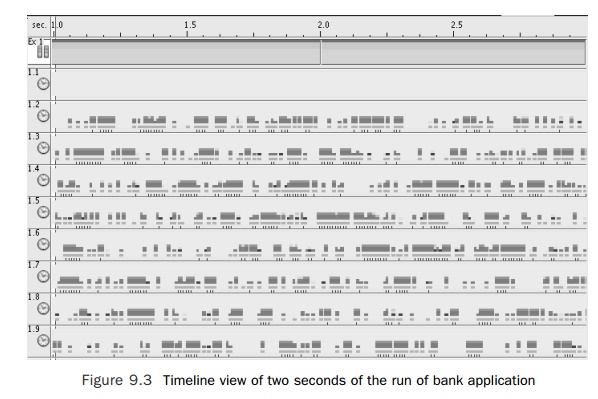
When run with a single thread, the program completes in about nine
seconds. When run with eight threads on the same platform, it takes about five
seconds to complete. The timeline view of the run of the application, shown in
Figure 9.3, indicates the problem. The figure shows two seconds from the
five-second run. Although all the threads are active some of the time, they are
inactive for significant portions of the time. The inac-tivity is represented
in the timeline view as gaps.
Looking at the profile, from the run of the
application with eight threads, the user time is not significantly different
from when it is run with a single thread. This indicates that the amount of
work performed is roughly the same. The one place where the pro-files differ is
in the amount of time spent in user locks. Listing 9.8 shows the profile from
the eight-way run. This shows that the eight threads accumulate about 10
seconds of time spent, in __lwp_park(), parked
waiting for user locks.
Listing 9.8 Profile
of Bank Application Run with Eight Threads
Excl. Excl. Name
User
CPU User Lock
sec. sec.
8.136 10.187 <Total>
1.811 0. rand_mt
1.041 0. atomic_cas_32
0.991 0. mutex_lock_impl
0.951 0. move
0.881 0. mutex_unlock
0.841 0. experiment
0.520 0. mutex_trylock_adaptive
0.490 0. rand_r
0.350 0. sigon
0.160 0. mutex_unlock_queue
0.070 0. mutex_lock
0.020 10.187 __lwp_park
On Solaris, the tool plockstat can be used to identify which locks are hot. Listing 9.9 shows the
output from plockstat. This
output indicates the contended locks. In this case, it is the lock named mutex in the routine move().
Listing 9.9 Output
from plockstat Indicating Hot Lock
% plockstat
./a.out 8 plockstat: pid 13970 has exited
Mutex
block
Count nsec Lock Caller
428
781859525 a.out`mutex a.out`move+0x14
Alternatively, the call stack can be examined to
identify the routine contributing to this time. Using either method, it is
relatively quick to identify that particular contended lock.
In this banking example, there are multiple branches,
and all account activity is restricted to occurring within a single branch. An
obvious solution is to provide a single mutex lock per branch. This will enable
one thread to lock up a transaction on a single branch, while other threads
continue to process transactions at other branches. Listing 9.10 shows the
modified code.
Listing 9.10 Bank
Example Modified So That Each Branch Has a Private Mutex Lock
#include <stdlib.h> #include
<strings.h> #include <pthread.h>
#define ACCOUNTS 256 #define BRANCHES 128
int
account[BRANCHES][ACCOUNTS];
pthread_mutex_t mutex[BRANCHES];
void
move( int branch, int from, int to, int value )
{
pthread_mutex_lock(
&mutex[branch] ); account[branch][from] -= value; account[branch][to] +=
value; pthread_mutex_unlock( &mutex[branch] );
}
void
*experiment( void *param )
{
unsigned
int seed = 0;
int
count = 10000000 / (int)param; for( int i=0; i<count; i++ )
{
int row = rand_r(&seed)
& (BRANCHES-1);
int
from = rand_r(&seed) &
(ACCOUNTS-1);
int to = rand_r(&seed)
& (ACCOUNTS-1);
move(
row, from, to, 1 );
}
}
int
main( int argc, char* argv[] )
{
pthread_t
threads[64];
memset(
account, 0, sizeof(account) ); int nthreads = 8;
if
( argc > 1 ) { nthreads = atoi( argv[1] ); }
for(
int i=0; i<BRANCHES; i++ )
pthread_mutex_init(
&mutex[i], 0 );
for(
int i=0; i<nthreads; i++ )
{
pthread_create(
&threads[i], 0, experiment, (void*)nthreads );
}
for(
int i=0; i<nthreads; i++ )
{
pthread_join(
threads[i], 0 );
}
for(
int i=0; i<BRANCHES; i++ )
pthread_mutex_destroy(
&mutex[i] );
return
0;
}
With this change in the application, the original runtime remains at
about nine sec-onds, but the runtime with eight threads drops to just over one
second. This is the expected degree of scaling.
It is interesting to compare the scaling of three different
configurations of the bank example. Figure 9.4 shows the scaling of the
original code, with 128 branches and a sin-gle mutex, from one to eight
threads; the scaling of the code with 128 branches, each with its own mutex; and
the code that shows the scaling if there were only four branches, each with a
single mutex.
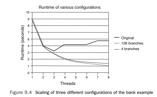
One point worth noting is that even the original
code shows some limited degree of scaling going from one to three threads. This
indicates that it is relatively easy to get some amount of scaling from most
applications. However, the scaling rapidly degrades when run with more than
three threads. Perhaps surprisingly, there is little difference in scaling
between provided 128 mutex locks or providing four. This is perhaps not as
sur-prising when considered in the context of the original mutex lock that
provides the ability to scale to three times the original thread count. It
might, therefore, be expected that four mutex locks might be sufficient to scale
the code to eight to twelve threads, which is in fact what is revealed if the
data collection is extended beyond eight threads.
Scaling
of Library Code
Issues with scaling are not restricted to just the application. It is
not surprising to find scaling issues in code provided in libraries. One of the
most fundamental library routines is the memory allocation provided by malloc() and free(). The
code shown in Listing 9.11 represents a very simple benchmark of malloc() performance as the number of threads increases. The benchmark creates a
number of threads, and each thread repeatedly allocates and frees a chunk of
1KB memory. The application completes after a fixed number of malloc() and free() calls
have been completed by the team of threads.
Listing 9.11 Code to Testing Scaling of malloc() and free()
#include <stdlib.h> #include
<pthread.h>
int nthreads;
void *work( void * param )
{
int count = 1000000 / nthreads; for( int i=0;
i<count; i++ )
{
void *mem =
malloc(1024); free( mem );
}
}
int main( int argc, char*argv[] )
{
pthread_t thread[50]; nthreads = 8;
if ( argc > 1 ) { nthreads = atoi( argv[1] ); }
for( int i=0; i<nthreads; i++ )
{
pthread_create( &thread[i], 0, work, 0 );
}
for( int i=0; i<nthreads; i++ )
{
pthread_join( thread[i], 0 );
}
return 0;
}
Suppose a default implementation of malloc() and free() uses a
single mutex lock to ensure that only a single thread can ever allocate or
deallocate memory at any one time. This implementation will limit the scaling
of the test code. The code is serialized, so performance will not improve with
multiple threads. Consider an alternative malloc() that uses a different algorithm. Each thread has its own heap of
memory, so it does not require a mutex lock. This alternative malloc() scales as the number of threads increases. Figure 9.5 shows the runtime
of the application in seconds using the two malloc() implementations as a function of the number of threads.
As expected, the default implementation does not scale, so the runtime
does not improve. The increase in runtime is because of more threads contending
for the single mutex lock. The alternative implementation shows very good
scaling. As the number of threads increases, the runtime of the application
decreases.
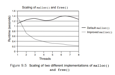
There is an interesting, though perhaps not
surprising, observation to be made from the performance of the two
implementations of malloc() and free(). For the single-threaded case, the default malloc() provides better performance than the alternative implementation. The
algorithm that provides improved scaling also adds a cost to the
single-threaded situation; it can be hard to produce an algorithm that is fast
for the sin-gle-threaded case and scales well with multiple threads.
If we return to the Mandelbrot example used in Chapter 7, “Using
Automatic Parallel-ization and OpenMP,” we made the work run in parallel by
having each thread compute a different range of iterations. A grid of 4,000 by
4,000 pixels was used, so there was plenty of work to be performed by each
thread. On the other hand, if we were comput-ing a grid of 64 by 64 pixels,
then using the same scheme we would not get scaling beyond 64 threads; each
thread would be able to compute a single row of the image.
Of course, the parallelization scheme could be
modified so that there was a single outer loop that iterated over the range 0
to 64 ∗ 64 = 4096. Listing 9.12 shows
the modified outer loop nest. With this modification, the maximum theoretical
thread count reaches 4,096. It is likely that, for this example on standard
hardware, the synchronization costs would dwarf the cost of the computation
long before 4,096 threads were reached.
Listing 9.12 Merging
Two Outer Loops to Provide More Parallelism
#pragma omp parallel for
for( int i=0; i<64*64; i++ )
{
y = i % SIZE;
x
= i / SIZE;
double xv = ( (double)x - (SIZE/2) ) / (SIZE/4);
double yv = ( (double)y - (SIZE/2) ) / (SIZE/4); matrix[x][y] = inSet( xv, yv
);
}
Of course, it is not uncommon to find that
scalability is limited by the number of iterations performed by the outer loop.
We have already met the OpenMP collapse clause,
which tells the compiler to perform this loop merge, as shown in Listing 9.13.
Listing 9.13 Using
the OpenMP collapse Directive
#pragma omp parallel for collapse(2) for( int x=0;
x<64; x++ )
for( int y=0; y<64; y++ )
{
double xv = ( (double)x – (SIZE/2) ) / (SIZE/4);
double yv = ( (double)y – (SIZE/2) ) / (SIZE/4); matrix[x][y] = inSet( xv, yv
);
}
However, if this code were to run with perfect
scaling on 4,096 processors, then there would be no further opportunities for
parallelization. If you recall, the routine inSet() has an iteration-carried dependence, so it cannot be parallelized, and
we have exhausted all the parallelism available at the call site.
The only options to extract further parallelism in
this particular instance would be to search for opportunities outside of this
part of the problem. The easiest thing to do would be to increase the size of
the problem; if there are spare threads, this might com-plete in the same
amount of time and end up being more useful.
The problem size can also be considered as
equivalent to the precision of the calcula-tion. It may be possible to use a
larger number of processors to provide a result with more precision. Consider
the example of numerical integration using the trapezium rule shown in Listing
9.14.
Listing 9.14 Numerical Integration Using the Trapezium Rule
#include <math.h> #include <stdio.h>
double function( double value )
{
return sqrt( value );
}
double integrate( double start, double end, int intervals )
{
double area = 0;
double range = ( end – start ) / intervals; for(
int i=1; i<intervals; i++ )
{
double pos = i*range + start; area += function( pos
);
}
area += ( function(start) + function(end) ) / 2; return range * area;
}
int
main()
{
for( int i=1; i<500; i++ )
{
printf( "%i intervals %8.5f value\n", i, integrate( 0, 1, i )
);
}
return 0;
}
The code calculates the integral of sqrt(x) over the range 0 to 1. The result of this calculation is the value
two-thirds. The time that the calculation takes depends on the number of steps
used; the smaller the step, the more accurate the result.
The example illustrates this very nicely when it is
run. When one step is used, the function calculates a value of 0.5 for the
integral. Once a few more steps are being used, it calculates a value of
0.66665. The more steps used, the greater the precision. As the number of steps
increases, there becomes more opportunity to spread the work over multiple
threads.
The actual computation time is minimal, so from
that perspective, the operation is not one that naturally needs to be sped up.
However, the calculation of the interval is clearly a good candidate for parallelization.
The only complication is the reduction implicit in calculating the value of the
variable area. It is
straightforward to parallelize the integration code using OpenMP, as shown in
Listing 9.15.
Listing 9.15 Numerical
Integration Code Parallelized Using OpenMP
double
integrate( double start, double end, int intervals )
{
double area = 0;
double range = ( end – start ) / intervals;
#pragma omp
parallel for reduction( +: area )
for( int i=1; i<intervals; i++ )
{
double pos = i*range + start; area += function( pos
);
}
area += ( function(start) + function(end) ) / 2;
return range * area ;
}
The other way of uncovering further opportunities
for parallelization, in the event of insufficient work, is to look at how the
results of the parallel computation are being used. Returning to the Mandelbrot
example, it may be the case that the computation is providing a single frame in
an animation. If this were the case, then the code could be parallelized at the
frame level, which may provide much more concurrent work.
Algorithmic
Limit
Algorithms have different abilities to scale to multiple processors. If
we return to dis-cussing sorting algorithms, bubble sort is an inherently
serial process. Each iteration through the list of elements that require
sorting essentially picks a single element and bubbles that element to the top.
It is possible to generalize this algorithm to a
parallel version called the odd-even sort.
This sort uses two alternate phases of sorting. In the first phase, all the
even elements are compared with the adjacent odd element. If they are in the
wrong order, then the two elements are swapped. In the second phase, this is
repeated with each odd element com-pared to the adjacent even element. This can
be considered as in the first phase compar-ing the pair of elements (0,1),
(2,3), and so on, and performing a swap between the elements as necessary. In
the second phase, the pairs are the elements (1,2), (3,4), and so on. In both
phases, each element is part of a single pair, so all the pairs can be computed
in parallel, using multiple threads, and the two elements in each pair can be
reordered without requiring any locks.
Obviously, better sorting algorithms are available.
The most obvious next step is the quicksort. The usual implementation of this
algorithm is serial, but it actually lends itself to a parallel implementation
because it recursively sorts shorter independent lists of val-ues. When
parallelized using tasks, each task performs computation on a distinct range of
elements, so there is no requirement for synchronization between the tasks. The
code shown in Listing 9.16 demonstrates how a parallel version of quicksort
could be imple-mented using OpenMP. The code is called through the quick_sort() routine. This code starts off the parallel region that contains the
entire algorithm but uses only a single thread to perform the initial pass. The
initial thread is responsible for creating additional tasks that will be
undertaken by other available threads.
Listing 9.16 Quicksort
Parallelized Using OpenMP
#include <stdio.h> #include <stdlib.h>
void setup( int * array,int len )
{
for
( int i=0; i<len; i++ )
{
array[i]
= (i*7 - 3224) ^ 20435;
}
}
void
quick_sort_range( int * array, int lower, int upper )
{
int
tmp;
int
mid = ( upper + lower ) / 2; int pivot = array[mid];
int
tlower = lower, tupper = upper; while ( tlower <= tupper )
{
while
( array[tlower] < pivot ) { tlower++; } while ( array[tupper] > pivot ) {
tupper--; } if ( tlower <= tupper )
{
tmp = array[tlower];
array[tlower] = array[tupper];
array[tupper] = tmp;
tupper--;
tlower++;
}
}
#pragma
omp task shared(array) firstprivate(lower,tupper)
if
( lower < tupper ) { quick_sort_range( array, lower, tupper ); }
#pragma
omp task shared(array) firstprivate(tlower,upper)
if
( tlower < upper ) { quick_sort_range( array, tlower, upper ); }
}
void
quick_sort( int *array, int elements )
{
#pragma
omp parallel
{
#pragma
omp single nowait quick_sort_range( array, 0, elements );
}
}
void
main()
{
int
size = 10*1024*1024;
int
* array = (int*)malloc( sizeof(int) * size ); setup( array, size);
quick_sort(
array, size-1 );
}
To summarize this discussion, some algorithms are
serial in nature, so to parallelize an application, the algorithm may need to
change. Not all parallel algorithms will be equally effective. Critical
characteristics are the number of threads an algorithm scales to and the amount
of overhead that the algorithm introduces.
In the context of the previous discussion, bubble
sort is serial but can be generalized to an odd-even sort. This makes better
use of multiple threads but is still not a very effi-cient algorithm. Changing
the algorithm to a quick sort provides a more efficient algo-rithm that still
manages to scale to many threads.
In this particular instance, we have been fortunate
in that our parallel algorithm also happened to be more efficient than the
serial version. This need not always be the case. It will sometimes be the case
that the parallel algorithm scales well, but at the cost of lower serial
performance. In these instances, it is worth considering whether both
algo-rithms need to be implemented and a runtime selection made as to which is
the more efficient.
There is another approach to algorithms that is not
uncommon in some application domains, particularly those where the computation
is performed across clusters with significant internode communication costs.
This is to use an algorithm that iteratively converges. The number of
iterations required depends on the accuracy requirements for the calculation.
This provides an interesting tuning mechanism for parallelizing the algorithm.
It is probably easiest to describe this with an
example. Suppose the problem is to model the flow of a fluid along an
obstructed pipe. It is easy to split the pipe into multiple sections and
allocate a set of threads to perform the computation for each sec-tion.
However, the results for one section will depend on the results for the
adjacent sections. So, the true calculation requires a large volume of data to
be exchanged at the intersections.
This exchange of data would serialize the
application and limit the amount of scaling that could be achieved. One way
around this is to approximate the values from the adja-cent sections and refine
those approximations as the adjacent sections refine their results. In this
way, it is possible to make the computations nearly independent of each other.
The cost of this approximation is that it will take more iterations of
the solver for it to converge on the correct answer.
This kind of approach is often taken with programs
run on clusters where there is significant cost associated with exchanging data
between two nodes. The approximations enable each node to continue processing
in parallel. Despite the increased number of iterations, this approach can lead
to faster solution times.
Related Topics