Chapter: Introduction to the Design and Analysis of Algorithms : Limitations of Algorithm Power
Challenges of Numerical Algorithms
Challenges of Numerical Algorithms
Numerical analysis is usually described as the branch of computer
science con-cerned with algorithms for solving mathematical problems. This
description needs an important clarification: the problems in question are
problems of “continuous” mathematics—solving equations and systems of
equations, evaluating such func-tions as sin x and ln x, computing integrals, and so on—as opposed to
problems of discrete mathematics dealing with such structures as graphs, trees,
permutations, and combinations. Our interest in efficient algorithms for
mathematical problems stems from the fact that these problems arise as models
of many real-life phe-nomena both in the natural world and in the social
sciences. In fact, numerical analysis used to be the main area of research,
study, and application of computer science. With the rapid proliferation of
computers in business and everyday-life applications, which deal primarily with
storage and retrieval of information, the relative
importance of numerical analysis has shrunk in the last 30 years. However, its applications, enhanced by the power
of modern computers, continue to expand in all areas of fundamental research
and technology. Thus, wherever one’s inter-ests lie in the wide world of modern
computing, it is important to have at least some understanding of the special
challenges posed by continuous mathematical problems.
We are not going to discuss the variety of difficulties posed by
modeling, the task of describing a real-life phenomenon in mathematical terms.
Assuming that this has already been done, what principal obstacles to solving a
mathematical problem do we face? The first major obstacle is the fact that most
numerical analy-sis problems cannot be solved exactly.4 They have to be solved
approximately, and this is usually done by replacing an infinite object by a
finite approximation. For example, the value of ex at a given point x can be computed by approximating its infinite
Taylor’s series about x = 0 by a finite sum of its first terms, called
the nth-degree Taylor polynomial:
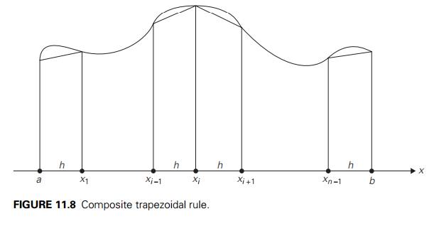
To give another example, the definite integral of a function can be
approximated by a finite weighted sum of its values, as in the composite
trapezoidal rule that you might remember from your calculus class:
where h = (b − a)/n,
xi = a + ih for i = 0, 1, . . . , n (Figure 11.8).
The errors of such approximations are called truncation errors. One of
the major tasks in numerical analysis is to estimate the magnitudes of
truncation
errors. This is typically done by using calculus tools, from
elementary to quite advanced. For example, for approximation (11.6) we have
where M = max eξ on the segment with the endpoints at 0 and x. This formula makes it possible to determine
the degree of Taylor’s polynomial needed to guar-antee a predefined accuracy
level of approximation (11.6).
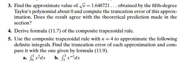
For example, if we want to compute e0.5 by formula (11.6) and
guarantee the truncation error to be smaller than 10−4, we can proceed as follows. First, we estimate M of formula (11.8):
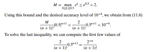
to see that the smallest
value of n for which this inequality
holds is 5.
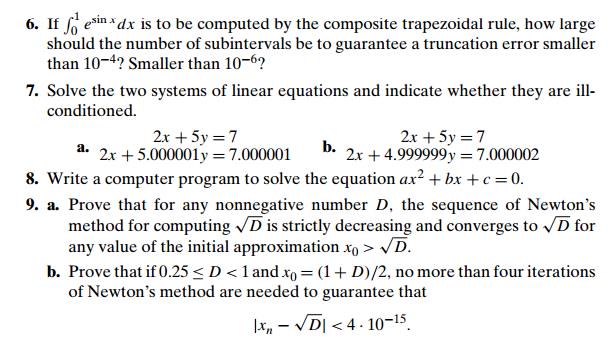
Similarly, for approximation (11.7), the standard bound of the
truncation error is given by the inequality
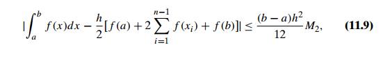
where M2 = max |f (x)| on the interval a ≤ x ≤ b. You are asked to use this
inequality in the exercises for this section (Problems 5 and 6).
The other type of errors, called round-off errors, are
caused by the limited accuracy with which we can represent real numbers in a
digital computer. These errors arise not only for all irrational numbers
(which, by definition, require an infinite number of digits for their exact
representation) but for many rational numbers as well. In the overwhelming
majority of situations, real numbers are represented as floating-point numbers,
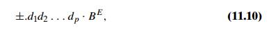
where B is the number base, usually 2 or 16 (or, for
unsophisticated calculators,
10); d1, d2, .
. . , dp are digits (0 ≤ di <
B for i = 1, 2, . . . , p and d1 > 0 unless the number is 0) representing together the fractional part of
the number and called
its mantissa; and E is an integer exponent with the range
of values approximately symmetric about 0.
The accuracy of the
floating-point representation depends on the number of significant digits p in representation (11.10). Most computers
permit two or even three levels of precision: single precision
(typically equivalent to between 6 and 7 significant decimal digits), double
precision (13 to 14 significant decimal digits), and extended
precision (19 to 20 significant decimal digits). Using higher-precision
arithmetic slows computations but may help to overcome some of the problems
caused by round-off errors. Higher precision may need to be used only for a
particular step of the algorithm in question.
As with an approximation of any kind, it is important to
distinguish between the absolute error and the relative
error of representing a number α∗ by its approximation α:
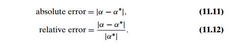
(The relative error is undefined if α∗ = 0.)
Very large and very small numbers cannot be represented in
floating-point arithmetic because of the phenomena called overflow and
underflow, respec-tively. An overflow happens when an arithmetic operation
yields a result out-side the range of the computer’s floating-point numbers.
Typical examples of overflow arise from the multiplication of large numbers or
division by a very small number. Sometimes we can eliminate this problem by
making a simple change in the order in which an
Underflow occurs when the
result of an operation is a nonzero fraction of such a small magnitude that it
cannot be represented as a nonzero floating-point number. Usually, underflow
numbers are replaced by zero, but a special signal is generated by hardware to
indicate such an event has occurred.
It is important to remember
that, in addition to inaccurate representation of numbers, the arithmetic
operations performed in a computer are not always exact, either. In particular,
subtracting two nearly equal floating-point numbers may cause a large increase
in relative error. This phenomenon is called subtractive cancellation.
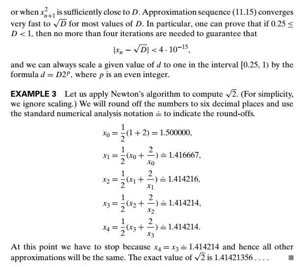
EXAMPLE
1 Consider two irrational numbers
α∗ = π = 3.14159265 . . . and β∗ = π − 6 . 10−7 = 3.14159205 . . .
represented by floating-point numbers α = 0.3141593 . 101 and β = 0.3141592 . 101, respectively. The relative errors of these
approximations are small:
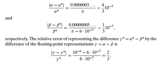
which is very large for a relative error despite quite accurate
approximations for both α and β.
Note that we may get a
significant magnification of round-off error if a low-accuracy difference is
used as a divisor. (We already encountered this problem in discussing Gaussian
elimination in Section 6.2. Our solution there was to use partial pivoting.)
Many numerical algorithms involve thousands or even millions of arithmetic
operations for typical inputs. For such algorithms, the propagation of
round-off errors becomes a major concern from both the practical and
theoretical standpoints. For some algorithms, round-off errors can propagate
through the algorithm’s operations with increasing effect. This highly
undesirable property of a numerical algorithm is called instability. Some
problems exhibit such a high level of sensitivity to changes in their input
that it is all but impossible to design a stable algorithm to solve them. Such
problems are called ill-conditioned.
EXAMPLE
2 Consider the following system of two linear equations in two unknowns:
1.001x + 0.999y = 2
0.999x + 1.001y = 2
Its only solution is x = 1,
y = 1. To see how sensitive this system is to small
changes to its right-hand side, consider the system with the same coefficient
matrix but slightly different right-hand side values:
1.001x + 0.999y = 2.002 0.999x + 1.001y = 1.998.
The only solution to this
system is x = 2,
y = 0, which is quite far from
the solution to the previous system. Note that the coefficient matrix of this
system is close to being singular (why?). Hence, a minor change in its
coefficients may yield a system with either no solutions or infinitely many
solutions, depending on its right-hand-side values. You can find a more formal
and detailed discussion of how we can measure the degree of ill-condition of
the coefficient matrix in numerical analysis textbooks (e.g., [Ger03]).
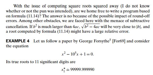
We conclude with a well-known
problem of finding real roots of the quadratic equation
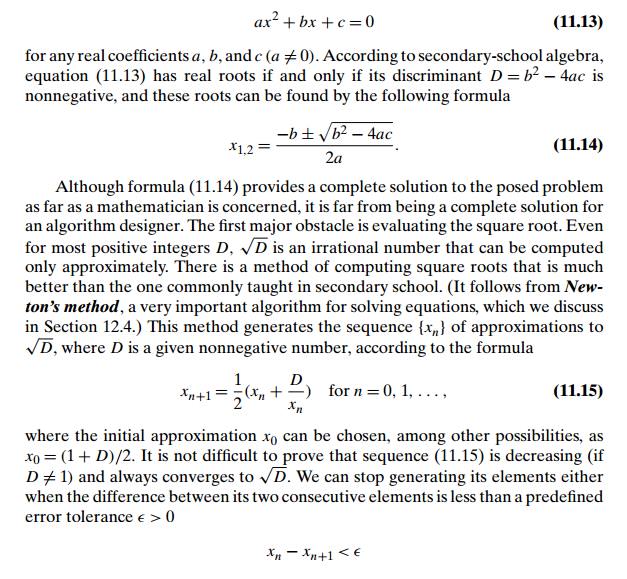
(The case of b = 0 can be considered with either of the other
two cases.)
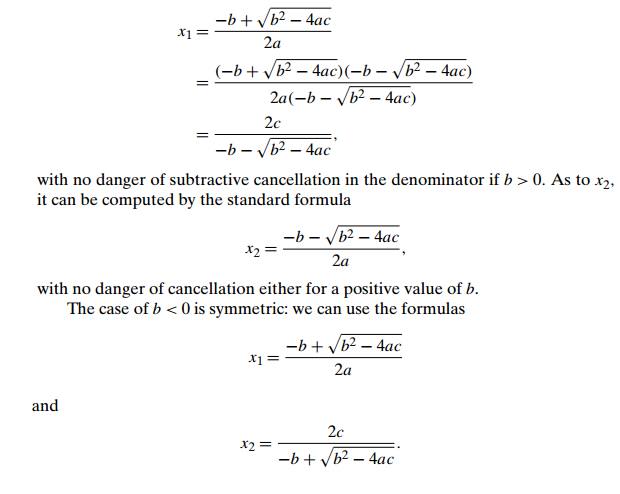
There are several other
obstacles to applying formula (11.14), which are re-lated to limitations of
floating-point arithmetic: if a is very small, division by a can cause an overflow; there seems to be no
way to fight the danger of subtractive cancellation in computing b2 − 4ac other than calculating it
with double precision; and so on. These problems have been overcome by William
Kahan of the Univer-sity of Toronto (see [For69]), and his algorithm is
considered to be a significant achievement in the history of numerical
analysis.
Hopefully, this brief
overview has piqued your interest enough for you to seek more information in
the many books devoted exclusively to numerical algorithms. In this book, we
discuss one more topic in the next chapter: three classic methods for solving
equations in one unknown.
Exercises 11.4
Some textbooks define the
number of significant digits in the approximation of number α∗ by number α as the largest nonnegative integer k for which
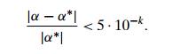
According to this definition,
how many significant digits are there in the approximation of π by
3.1415?b. 3.1417?
If α = 1.5 is known to approximate
some number α∗ with the absolute error not exceeding 10−2, find
the range of possible values of α∗.
the range of the relative
errors of these approximations.
![]() 10. Apply four iterations of Newton’s method to
compute 3 and estimate the absolute and relative errors of this approximation.
10. Apply four iterations of Newton’s method to
compute 3 and estimate the absolute and relative errors of this approximation.
SUMMARY
Given a class of algorithms
for solving a particular problem, a lower
bound indicates the best possible efficiency any algorithm from this class can have.
A trivial lower bound is based on counting the number of items in the
problem’s input that must be processed and the number of output items that need
to be produced.
An information-theoretic lower bound is usually obtained through a
mecha-nism of decision trees. This
technique is particularly useful for comparison-based algorithms for sorting
and searching. Specifically:
Any general comparison-based
sorting algorithm must perform at least log2 n! ≈ n log2 n key comparisons in the worst case.
Any general comparison-based
algorithm for searching a sorted array must perform at least log2(n + 1) key comparisons in the worst
case.
The adversary method for establishing lower bounds is based on
following the logic of a malevolent adversary who forces the algorithm into the
most time-consuming path.
A lower bound can also be
established by reduction, i.e., by
reducing a problem with a known lower bound to the problem in question.
Complexity theory seeks to classify problems
according to their computational complexity.
The principal split is between tractable
and intractable problems
problems that can and cannot
be solved in polynomial time, respectively. For purely technical reasons,
complexity theory concentrates on decision
problems, which are problems with
yes/no answers.
The halting problem is an example of an undecidable decision problem; i.e., it cannot be solved by any
algorithm.
P is the class of all decision problems that can
be solved in polynomial time. NP is the class of all decision problems whose randomly guessed
solutions can be verified in
polynomial time.
Many important problems in NP (such as the Hamiltonian circuit
problem) are known to be NP-complete:
all other problems in NP are
reducible to such a problem in polynomial time. The first proof of a problem’s NP-completeness was published by S. Cook
for the CNF-satisfiability problem.
It is not known whether P = NP
or P is just a proper subset of NP. This question is the most important unresolved
issue in theoretical computer science. A discovery of a polynomial-time
algorithm for any of the thousands of known NP-complete
problems would imply that P = NP.
Numerical analysis is a branch of computer science dealing with
solving continuous mathematical
problems. Two types of errors occur in solving a majority of such problems:
truncation error and round-off error. Truncation
errors stem from replacing infinite
objects by their finite approximations.
Round-off errors are due to inaccuracies of representing numbers
in a digital computer.
Subtractive cancellation happens as a result of subtracting two
near-equal floating-point numbers. It
may lead to a sharp increase in the relative round-off error and therefore
should be avoided (by either changing the expression’s form or by using a
higher precision in computing such a difference).
Writing a general computer program for solving
quadratic equations ax2 + bx
+ c = 0 is a difficult task. The
problem of computing square roots can be solved by utilizing Newton’s method; the problem of subtractive cancellation can be
dealt with by using different formulas depending on whether coefficient b is positive or negative and by computing the
discriminant b2 − 4ac
with double precision.
Related Topics