Breadth First Search

Explain in detail about Breadth First Search

This strategy for searching a graph is known as breadth-first search. It operates by processing vertices in layers: The vertices closest to the start are evaluated first, and the most distant vertices are evaluated last. This is much the same as a level-order traversal for trees.

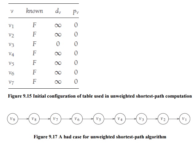
Given this strategy, we must translate it into code. Figure 9.15 shows the initial configuration of the table that our algorithm will use to keep track of its progress. For each vertex, we will keep track of three pieces of information. First, we will keep its distance from s in the entry dv. Initially all vertices are unreachable except for s, whose path length is 0. The entry in pv is the bookkeeping variable, which will allow us to print the actual paths. The entry known is set to true after a vertex is processed. Initially, all entries are not known, including the start vertex. When a vertex is marked known, we have

a guarantee that no cheaper path will ever be found, and so processing for that vertex is essentially complete. The basic algorithm can be described in Figure 9.16. The algorithm n below mimics the diagrams by declaring as known the vertices at distance d = 0, then d = 1, then d = 2, and so on, and setting all the adjacent vertices w that still have dw = ∞to a distance dw = d + 1.

Pseudocode for unweighted shortest-path algorithm

void Graph::unweighted( Vertex s )

{

for each Vertex v

{

v.dist = INFINITY;

v.known = false;

}

s.dist = 0;

for( int currDist = 0; currDist < NUM_VERTICES; currDist++ )

for each Vertex v

if( !v.known && v.dist == currDist )

{

v.known = true;

for each Vertex w adjacent to v

if( w.dist == INFINITY )

{

w.dist = currDist + 1;

w.path = v;

}

}

}

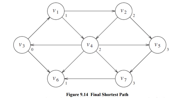
using the above algorithmBy tracing back through the pv variable, the actual path can be printed. We will seehow when we discuss the weighted case. The running time of the algorithm is O(|V|2), because of the doubly nested for loops. An obvious inefficiency is that the outside loop continues until NUM_VERTICES-1, even if all the vertices become known much earlier. Although an extra test could be made to avoid this, it does not affect the worst-case running time, as can be seen by generalizing what happens when the input is the graph in Figure 9.17 with start vertex v9. We can remove the inefficiency in much the same way as was done for topological sort. At any point in time, there are only two types of unknown vertices that have dv _=∞. Some have dv = currDist, and the rest have dv = currDist + 1. Because of this extra structure, it is very wasteful to search through the entire table to find a proper vertex. A very simple but abstract solution is to keep two boxes. Box #1 will have the unknown vertices with dv = currDist, and box #2 will have dv = currDist + 1.

The test to find an appropriate vertex v can be replaced by finding any vertex in box #1. After updating w (inside the innermost if block), we can add w to box #2. After the outermost for loop erminates, box #1 is empty, and box #2 can be transferred to box #1 for the next pass of the for loop. We can refine this idea even further by using just one queue. At the start of the pass, the queue contains only vertices of distance currDist. When we add adjacent vertices of distance currDist + 1, since they enqueue at the rear, we are guaranteed that they will not be processed until after all the vertices of distance currDist have been processed. After the last vertex at distance currDist dequeues and is processed, the queue only contains vertices of distance currDist + 1, so this process perpetuates. We merely need to begin the process by placing the start node on the queue by itself.

The refined algorithm is shown in Figure 9.18. In the pseudocode, we have assumed that the start vertex, s, is passed as a parameter. Also, it is possible that the queue might empty prematurely, if some vertices are unreachable from the start node. In this case, a distance of INFINITY will be reported for these nodes, which is perfectly reasonable. Finally, the known data member is not used; once a vertex is processed it can never enter the queue again, so the fact that it need not be reprocessed is implicitly marked. Thus, the known data member can be discarded. Figure 9.19 shows how the values on the graph we have been using are changed during the algorithm (it includes the changes that would occur to known if we had kept it). Using the same analysis as was performed for topological sort, we see that the running time is O(|E| + |V|), as long as adjacency lists are used.