Basic Concepts of Interprocedural Analysis

Basic Concepts

1 Call Graphs

2 Context Sensitivity

3 Call Strings

4 Cloning-Based Context-Sensitive Analysis

5 Summary-Based Context-Sensitive Analysis

6 Exercises for Section 12.1

In this section, we introduce call graphs — graphs that tell us which procedures can call which. We also introduce the idea of "context sensitivity," where data-flow analyses are required to take cognizance of what the sequence of procedure calls has been. That is, context-sensitive analysis includes (a synopsis of) the current sequence of activation records on the stack, along with the current point in the program, when distinguishing among different "places" in the program.

1. Call Graphs

A call graph for a program is a set of nodes and edges such that

1.  There is one node for each procedure in the program.

•2,.. There is one node for each call site, that is, a place in the program where a procedure is invoked.

3.  If call site c may call procedure p, then there is an edge from the node for c to the node for p.

Many programs written in languages like C and Fortran make procedure calls directly, so the call target of each invocation can be determined statically. In that case, each call site has an edge to exactly one procedure in the call graph. However, if the program includes the use of a procedure parameter or function pointer, the target generally is not known until the program is run and, in fact, may vary from one invocation to another. Then, a call site can link to many or all procedures in the call graph.

Indirect calls are the norm for object-oriented programming languages. In particular, when there is overriding of methods in subclasses, a use of method m may refer to any of a number of different methods, depending on the subclass of the receiver object to which it was applied. The use of such virtual method invocations means that we need to know the type of the receiver before we can determine which method is invoked.

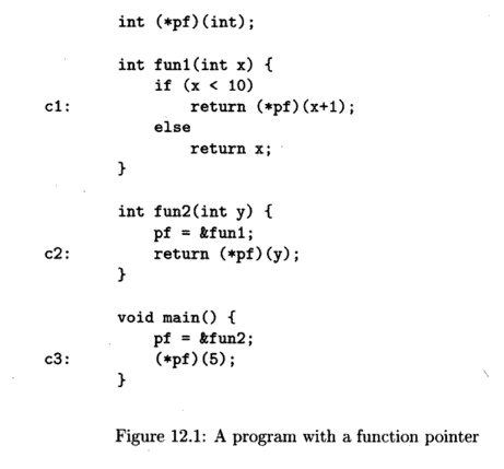
Example 1 2 . 1 : Figure 12.1 shows a C program that declares pf to be a global pointer to a function whose type is "integer to integer." There are two functions of this type, f unl and f un2, and a main function that is not of the type that pf points to. The figure shows three call sites, denoted c l , c2, and c3; the labels are not part of the program.

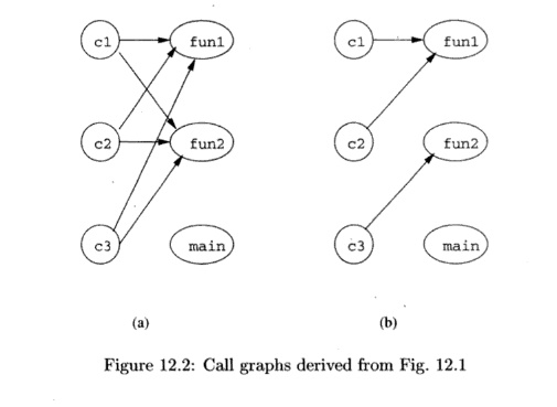
The simplest analysis of what pf could point to would simply observe the types of functions. Functions funl and fun2 are of the same type as what pf points to, while main is not. Thus, a conservative call graph is shown in Fig. 12.2(a). A more careful analysis of the program would observe that pf is made to point to fun2 in main and is made to point to funl in fun2. But there are no other assignments to any pointer, so, in particular, there is no way for pf to point to main. This reasoning yields the same call graph as Fig. 12.2(a).

An even more precise analysis would say that at c3, it is only possible for pf to point to f un2, because that call is preceded immediately by that assignment to pf. Similarly, at c2 it is only possible for pf to point to f u n l . As a result, the initial call to funl can come only from fun2, and funl does not change pf, so whenever we are within funl, pf points to funl . In particular, at c l , we can be sure pf points to f u n l . Thus, Fig. 12.2(b) is a more precise, correct call graph.

In general, the presence of references or pointers to functions or methods requires us to get a static approximation of the potential values of all procedure parameters, function pointers, and receiver object types. To make an accurate approximation, interprocedural analysis is necessary. The analysis is iterative, starting with the statically observable targets. As more targets are discov-ered, the analysis incorporates the new edges into the call graph and repeats discovering more targets until convergence is reached.

2. Context Sensitivity

Interprocedural analysis is challenging because the behavior of each procedure is dependent upon the context in which it is called. Example 12.2 uses the problem of interprocedural constant propagation on a small program to illustrate the significance of contexts.

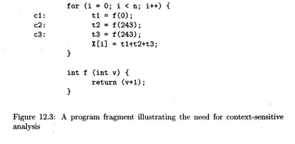
Example 12*2: Consider the program fragment in Fig. 12.3. Function / is invoked at three call sites: c l , c2 and c3 . Constant 0 is passed in as the actual parameter at c l , and constant 243 is passed in at c2 and c3 in each iteration; the constants 1 and 244 are returned, respectively. Thus, function / is invoked with a constant in each of the contexts, but the value of the constant is context-dependent.

As we shall see, it is not possible to tell that t l , t 2 , and t3 each are assigned constant values (and thus so is X[i)), unless we recognize that when called in context c l , / returns 1, and when called in the other two contexts, / returns 244. A naive analysis would conclude that / can return either 1 or 244 from any call. •

One simplistic but extremely inaccurate approach to interprocedural anal-ysis, known as context-insensitive analysis, is to treat each call and return statement as "goto" operations. We create a super control-flow graph where, besides the normal intraprocedural control flow edges, additional edges are cre-ated connecting

1. Each call site to the beginning of the procedure it calls, and

2. The return statements back to the call sites.¹

Assignment statements are added to assign each actual parameter to its corresponding formal parameter and to assign the returned value to the variable receiving the result. We can then apply a standard analysis intended to be used within a procedure to the super control-flow graph to find context-insensitive interprocedural results. While simple, this model abstracts out the important relationship between input and output values in procedure invocations, causing the analysis to be imprecise.

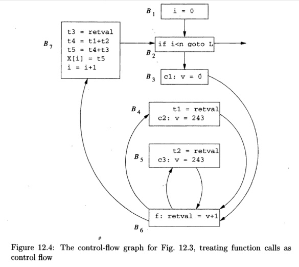
Example 1 2 . 3 : The super control-flow graph for the program in Fig. 12.3 is shown in Figure 12.4. Block BQ is the function /. Block B3 contains the call site c l ; it sets the formal parameter v to 0 and then jumps to the beginning of /, at BQ. Similarly, B4 and £5 represent the call sites c2 and c3, respectively. In £4, which is reached from the end of / (block BQ), we take the return value from / and assign it to t l . We then set formal parameter v to 243 and call / again, by jumping to B₆. Note that there is no edge from B3 to B4. Control must flow through / on the way from B3 to B4.

B5 is similar to B4. It receives the return from /, assigns the return value to t 2 , and initiates the third call to /. Block B7 represents the return from the third call and the assignment to X[i],

If we treat Fig. 12.4 as if it were the flow graph of a single procedure, then we would conclude that coming into BQ, V can have the value 0 or 243. Thus, the most we can conclude about r e t v a l is that it is assigned 1 or 244, but no other value. Similarly, we can only conclude about t l , t 2 , and t3 that they can each be either 1 or 244. Thus, X[i] appears to be either 3, 246, 489, or 732. In contrast, a context-sensitive analysis would separate the results for each of the calling contexts and produces the intuitive answer described in Example 12.2: tl is always 1, t2 and t3 are always 244, and X[i] is 489.

3. Call Strings

In Example 12.2, we can distinguish among the contexts by just knowing the call site that calls the procedure /. In general, a calling context is defined by the contents of the entire call stack. We refer to the string of call sites on the stack as the call string.

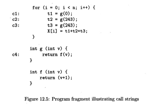
Example 1 2 . 4 : Figure 12.5 is a slight modification of Fig. 12.3. Here we have replaced the calls to / by calls to g, which then calls / with the same argument. There is an additional call site, c4, where g calls f.

There are three call strings to f: (cl, c4), (c2, c4), and (c3, c4). As we see in this example, the value of v in function f depends not on the immediate or last site c4 on the call string. Rather, the constants are determined by the first element in each of the call strings. •

Example 12.4 illustrates that information relevant to the analysis can be introduced early in the call chain. In fact, it is sometimes necessary to consider the entire call string to compute the most precise answer, as illustrated in Example 12.5.

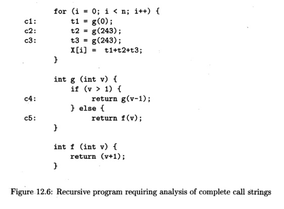
Example 1 2 . 5 : This example illustrates how the ability to reason about un bounded call strings can yield more precise results. In Fig. 12.6 we see that if g is called with a positive value c, then g will be invoked recursively c times. Each time g is called, the value of its parameter v decreases by 1. Thus, the value of g's parameter v in the context whose call string is c2(c4) ⁿ is 243 - n. The effect of g is thus to increment 0 or any negative argument by 1, and to return 2 on any argument 1 or greater.

There are three possible call strings for /. If we start with the call at c l , then g calls / immediately, so (cl, c5) is one such string. If we start at c2 or c3, then we call g a total of 243 times, and then call /. These call strings are (c2, c4, c 4 , . . . , c5) and (c3, c4, c 4 , . . . , c5), where in each case there are 242 c4's in the sequence. In the first of these contexts, the value of / ' s parameter v is 0, while in the other two contexts it is 1.

In designing a context-sensitive analysis, we have a choice in precision. For example, instead of qualifying the results by the full call string, we may just choose to distinguish between contexts by their k most immediate call sites. This technique is known as fc-limiting context analysis. Context-insensitive analysis is simply a special case of fc-limiting context analysis, where k is 0. We can find all the constants in Example 12.2 using a 1-limiting analysis and all the constants in Example 12.4 using a 2-limiting analysis. However, no ^-limiting analysis can find all the constants in Example 12.5, provided the constant 243 were replaced by two different and arbitrarily large constants.

Instead of choosing a fixed value k, another possibility is to be fully con-text sensitive for all acyclic call strings, which are strings that contain no re-cursive cycles. For call strings with recursion, we can collapse all recursive cycles, in order to bound the number of different contexts analyzed. In Ex-ample 12.5, the calls initiated at call site c2 may be approximated by the call string: (c2,c4*,c5) . Note that, with this scheme, even for programs without recursion, the number of distinct calling contexts can be exponential in the number of procedures in the program.

4. Cloning-Based Context-Sensitive Analysis

Another approach to context-sensitive analysis is to clone the procedure con-ceptually, one for each unique context of interest. We can then apply a context-insensitive analysis to the cloned call graph. Examples 12.6 and 12.7 show the equivalent of a cloned version of Examples 12.4 and 12.5, respectively. In real-ity, we do not need to clone the code, we can simply use an efficient internal representation to keep track of the analysis results of each clone.

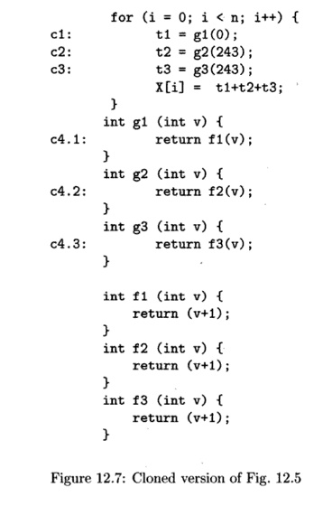
Example 12.6 : The cloned version of Fig. 12.5 is shown in Fig. 12.7. Because every calling context refers to a distinct clone, there is no confusion. For ex-ample, gl receives 0 as input and produces 1 as output, and g2 and g3 both receive 243 as input and produce 244 as output.

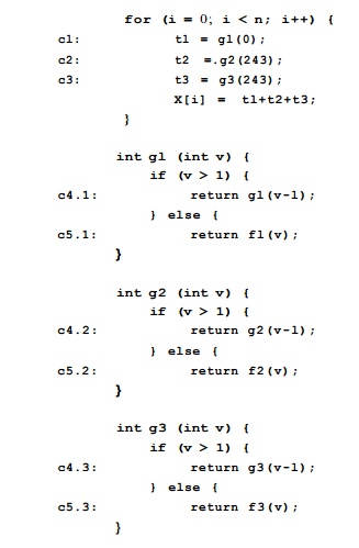
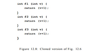
Example 1 2 . 7 : The cloned version of Example 12.5 is shown in Fig. 12.8. For procedure g, we create a clone to represent all instances of g that are first called from sites c l , c2, and c3 . In this case, the analysis would determine that the invocation at call site cl returns 1, assuming the analysis can deduce that with v = 0, the test v > 1 fails. This analysis does not handle recursion well enough to produce the constants for call sites c2 and c3, however.

5. Summary-Based Context-Sensitive Analysis

Summary-based interprocedural analysis is an extension of region-based anal-ysis. Basically, in a summary-based analysis each procedure is represented by a concise description ("summary") that encapsulates some observable behavior

of the procedure. The primary purpose of the summary is to avoid reanalyzing * a procedure's body at every call site that may invoke the procedure.

Let us first consider the case where there is no recursion. Each procedure is modeled as a region with a single entry point, with each caller-callee pair sharing

an outer-inner region relationship. The only difference from the intraprocedural version is that, in the interprocedural case, a procedure region can be nested inside several different outer regions.

The analysis consists of two parts:

1.                 A bottom-up phase that computes a transfer function to summarize the effect of a procedure, and

2.                 A top-down phase that propagates caller information to compute results of the callees.

To get fully context-sensitive results, information from different calling contexts must propagate down to the callees individually. For a more efficient, but less precise calculation, information from all callers can be combined, using a meet operator, then propagated down to the callees.

Example 12 . 8 : For constant propagation, each procedure is summarized by a transfer function specifying how it would propagate constants through its body. In Example 12.2, we can summarize / as a function that, given a constant c as an actual parameter to v, returns the constant c+1. Based on this information, the analysis would determine that t l , t 2 , and t3 have the constant values 1, 244, and 244, respectively. Note that this analysis does not suffer the inaccuracy due to unrealizable call strings.

Recall that Example 12.4 extends Example 12.2 by having g call /. Thus, we could conclude that the transfer function for g is the same as the transfer function for /. Again we conclude that t l , t 2 , and t3 have the constant values 1, 244, and 244, respectively.

Now, let us consider what is the value of parameter v in function / for Example 12,2. As a first cut, we can combine all the results for all calling contexts. Since v may have values 0 or 243, we can simply conclude that v is not a constant. This conclusion is fair, because there is no constant that can replace v in the code.

If we desire more precise results, we can compute specific results for contexts of interest. Information must be passed down from the context of interest to determine the context-sensitive answer. This step is analogous to the top-down pass in region-based analysis. For example, the value of v is 0 at call site cl and 243 at sites c2 and c3. To get the advantage of constant propagation within /, we need to capture this distinction by creating two clones, with the first specialized for input value 0 and the latter with value 243, as shown in Fig. 12.9.

With Example 12.8, we see that, in the end, if we wish to compile the code differently in different contexts, we still need to clone the code. The difference is that in the cloning-based approach, cloning is performed prior to the analysis, based on the call strings. In the summary-based approach, the cloning is performed after the analysis, using the analysis results as a basis.

Even if cloning is not applied, in the summary-based approach inferences about the effect of a called procedure are made accurately, without the problem of unrealizable paths.

Instead of cloning a function, we could also inline the code. Inlining has the additional effect of eliminating the procedure-call overhead as well.

We can handle recursion by computing the fixedpoint solution. In the pres-ence of recursion, we first find the strongly connected components in the call graph. In the bottom-up phase, we do not visit a strongly connected component unless all its successors have been visited. For a nontrivial strongly connected component, we iteratively compute the transfer functions for each procedure in the component until convergence is reached; that is, we iteratively update the transfer functions until no more changes occur.

6. Exercises for Section 12.1

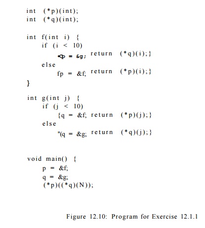
Exercise 1 2 . 1 . 1 : In Fig. 12.10 is a C program with two function pointers, p and q. N is a constant that could be less than or greater than 10. Note that the program results in an infinite sequence of calls, but that is of no concern for the purposes of this problem.

a) Identify all the call sites in this program.

b) For each call site, what can p point to? What can q point to?

c) Draw the call graph for this program.

d) Describe all the call strings for f and g.

Exercise 12 . 1 . 2 :        In Fig.         12.11 is a function id that is the "identity function";   it returns exactly what it is given as an argument. We also see a code fragment consisting of a branch and following assignment that sums x + y.

a)  Examining the code, what can we tell about the value of z at the end?

b)  Construct the flow graph for the code fragment, treating the calls to  id as control flow.

c) If we run a constant-propagation analysis, as in Section 9.4, on your flow graph from (b), what constant values are determined?

d) What are all the call sites in Fig. 12.11?

e) What are all the contexts in which id is called?

f) Rewrite the code of Fig. 12.11 by cloning a new version of id for each context in which it is called.

g) Construct the flow graph of your code from (f), treating the calls as control flow.

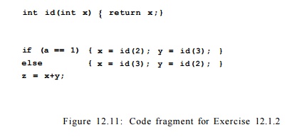
h)                Perform a constant-propagation analysis on your flow graph from (g). What constant values are determined now?