Chapter: Introduction to the Design and Analysis of Algorithms : Coping with the Limitations of Algorithm Power
Approximation Algorithms for the Knapsack Problem
Approximation
Algorithms for the Knapsack Problem
The knapsack problem, another
well-known NP-hard problem, was also intro-duced in Section 3.4:
given n items of known weights w1, . . . , wn and values v1, . . . , vn and a knapsack of weight capacity W, find the most valuable sub-set of the items
that fits into the knapsack. We saw how this problem can be solved by
exhaustive search (Section 3.4), dynamic programming (Section 8.2), and
branch-and-bound (Section 12.2). Now we will solve this problem by
approx-imation algorithms.
Greedy Algorithms for the Knapsack Problem We can
think of several greedy approaches
to this problem. One is to select the items in decreasing order of their
weights; however, heavier items may not be the most valuable in the set.
Alternatively, if we pick up the items in decreasing order of their value,
there is no guarantee that the knapsack’s capacity will be used efficiently.
Can we find a greedy strategy that takes into account both the weights and
values? Yes, we can, by computing the value-to-weight ratios vi/wi, i = 1, 2, . . .
, n, and selecting the items in decreasing order of
these ratios. (In fact, we already used this approach in designing the
branch-and-bound algorithm for the problem in Section 12.2.) Here is the
algorithm based on this greedy heuristic.
Greedy
algorithm for the discrete knapsack problem
Step 1 Compute the value-to-weight ratios ri = vi/wi, i = 1, . . . , n, for the items given.
Step 2 Sort the items in nonincreasing order of the ratios computed in
Step 1. (Ties can be broken
arbitrarily.)
Step 3 Repeat the following operation until no item is left in the sorted
list: if the current item on the
list fits into the knapsack, place it in the knapsack and proceed to the next
item; otherwise, just proceed to the next item.
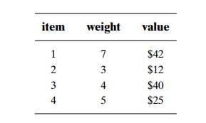
EXAMPLE
5 Let us consider the instance of the knapsack problem with the knapsack capacity 10 and the
item information as follows:
Computing the value-to-weight
ratios and sorting the items in nonincreasing order of these efficiency ratios
yields
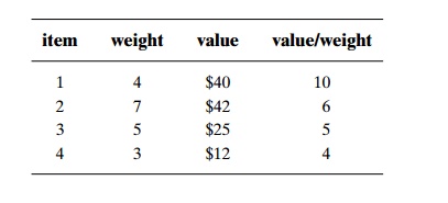
The greedy algorithm will
select the first item of weight 4, skip the next item of weight 7, select the
next item of weight 5, and skip the last item of weight 3. The solution
obtained happens to be optimal for this instance (see Section 12.2, where we
solved the same instance by the branch-and-bound algorithm).
Does this greedy algorithm
always yield an optimal solution? The answer, of course, is no: if it did, we
would have a polynomial-time algorithm for the NP-hard problem. In fact, the following example shows that no
finite upper bound on the accuracy of its approximate solutions can be given
either.
EXAMPLE
6
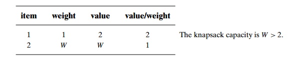
Since the items are already
ordered as required, the algorithm takes the first item and skips the second
one; the value of this subset is 2. The optimal selection con-sists of item 2
whose value is W. Hence, the accuracy ratio r(sa) of this approximate solution is W/2, which is unbounded above.
It is surprisingly easy to
tweak this greedy algorithm to get an approximation algorithm with a finite
performance ratio. All it takes is to choose the better of two alternatives:
the one obtained by the greedy algorithm or the one consisting of a single item
of the largest value that fits into the knapsack. (Note that for the instance
of the preceding example, the second alternative is better than the first one.)
It is not difficult to prove that the performance ratio of this enhanced
greedy
algorithm is 2. That is, the value of an optimal subset s∗ will never be more than
twice as large as the value of the subset sa obtained by this enhanced greedy algorithm,
and 2 is the smallest multiple for which such an assertion can be made.
It is instructive to consider
the continuous version of the knapsack problem as well. In this version, we are
permitted to take arbitrary fractions of the items given. For this version of
the problem, it is natural to modify the greedy algorithm as follows.
Greedy
algorithm for the continuous knapsack problem
Step 1 Compute the value-to-weight ratios vi/wi, i = 1, . . . , n, for the items given.
Step 2 Sort the items in nonincreasing order of the ratios computed in
Step 1. (Ties can be broken
arbitrarily.)
Step 3 Repeat the following operation until the knapsack is filled to its
full capacity or no item is left in
the sorted list: if the current item on the list fits into the knapsack in its
entirety, take it and proceed to the next item; otherwise, take its largest
fraction to fill the knapsack to its full capacity and stop.
For example, for the
four-item instance used in Example 5 to illustrate the greedy algorithm for the
discrete version, the algorithm will take the first item of weight 4 and then
6/7 of the next item on the sorted list to fill the knapsack to its full
capacity.
It should come as no surprise
that this algorithm always yields an optimal solution to the continuous
knapsack problem. Indeed, the items are ordered according to their efficiency
in using the knapsack’s capacity. If the first item on the sorted list has
weight w1 and value v1, no solution can use w1 units of capacity with a higher payoff than v1. If we cannot fill the knapsack with the first
item or its fraction, we should continue by taking as much as we can of the
second-most efficient item, and so on. A formal rendering of this proof idea is
somewhat involved, and we will leave it for the exercises.
Note also that the optimal
value of the solution to an instance of the contin-uous knapsack problem can
serve as an upper bound on the optimal value of the discrete version of the
same instance. This observation provides a more sophisti-cated way of computing
upper bounds for solving the discrete knapsack problem by the branch-and-bound
method than the one used in Section 12.2.
Approximation Schemes We now return to the discrete version of the
knap-sack problem. For this problem, unlike the traveling salesman problem,
there exist polynomial-time approximation schemes, which are
parametric families of algo-rithms that allow us to
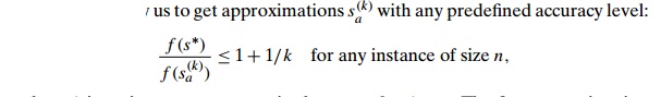
where k is an integer parameter in the range 0 ≤ k
< n. The first approximation scheme was suggested by S. Sahni in 1975
[Sah75]. This algorithm generates all subsets of k items or less, and for each one that fits into
the knapsack it adds the remaining items as the greedy algorithm would do
(i.e., in nonincreasing order of their value-to-weight ratios). The subset of
the highest value obtained in this fashion is returned as the algorithm’s
output.
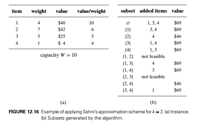
EXAMPLE
7 A small example of an approximation scheme with k = 2 is pro-vided in Figure
12.16. The algorithm yields {1, 3, 4}, which is the optimal solution for this
instance.
You can be excused for not
being overly impressed by this example. And, indeed, the importance of this
scheme is mostly theoretical rather than practical. It lies in the fact that,
in addition to approximating the optimal solution with any predefined accuracy
level, the time efficiency of this
algorithm is polynomial in n. Indeed, the total number of
subsets the algorithm generates before adding extra elements is
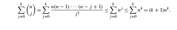
For each of those subsets, it
needs O(n) time to determine the
subset’s possible extension. Thus, the algorithm’s efficiency is in O(knk+1). Note that although it is polynomial in n, the time efficiency of Sahni’s scheme is
exponential in k. More sophisticated
approximation schemes, called fully polynomial schemes, do not
have this shortcoming. Among several books that discuss such algorithms, the
monographs [Mar90] and [Kel04] are especially recommended for their wealth of
other material about the knapsack problem.
Exercises 12.3
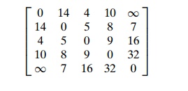
a. Apply the nearest-neighbor algorithm to the instance defined by the
inter-city distance matrix below. Start the algorithm at the first city,
assuming that the cities are numbered from 1 to 5.
b. Compute the accuracy ratio of this approximate solution.
a. Write pseudocode for the
nearest-neighbor algorithm. Assume that its
input is given by an n × n intercity distance matrix.
What is the time efficiency of the nearest-neighbor algorithm?
Apply the twice-around-the-tree algorithm to the graph in Figure
12.11a with a walk around the minimum spanning tree that starts at the same
vertex a but differs from the walk in
Figure 12.11b. Is the length of the obtained tour the same as the length of the
tour in Figure 12.11b?
Prove that making a shortcut of the kind used by the
twice-around-the-tree algorithm cannot increase the tour’s length in a
Euclidean graph.
What is the time efficiency class of the greedy algorithm for the
knapsack problem?
Prove that the performance ratio RA of the enhanced greedy algorithm for the
knapsack problem is equal to 2.
Consider the greedy algorithm for the bin-packing problem, which is
called the first-fit (FF ) algorithm:
place each of the items in the order given into the first bin the item fits in;
when there are no such bins, place the item in a new bin and add this bin to
the end of the bin list.
Apply FF to the instance
s1 = 0.4, s2 = 0.7, s3 = 0.2, s4 = 0.1, s5 = 0.5
and determine whether the
solution obtained is optimal.
Determine the worst-case time efficiency of FF .
Prove that FF is a
2-approximation algorithm.
The first-fit decreasing (FFD)
approximation algorithm for the bin-packing problem starts by sorting the items
in nonincreasing order of their sizes and then acts as the first-fit algorithm.
Apply FFD to the instance
s1 = 0.4, s2 = 0.7, s3 = 0.2, s4 = 0.1, s5 = 0.5
and determine whether the
solution obtained is optimal.
Does FFD always yield an
optimal solution? Justify your answer.
Prove that FFD is a 1.5-approximation algorithm.
Run an experiment to determine which of the two algorithms—FF or FFD—yields more accurate approximations on a random sample of the problem’s instances.
a. Design a simple
2-approximation algorithm for finding a minimum vertex cover (a vertex cover with the smallest number of vertices) in
a given graph.
Consider the following
approximation algorithm for finding a maximum independent set (an
independent set with the largest number of vertices) in a given graph. Apply the
2-approximation algorithm of part (a) and output all the vertices that are not
in the obtained vertex cover. Can we claim that this algorithm is a
2-approximation algorithm, too?
a. Design a polynomial-time
greedy algorithm for the graph-coloring prob-lem.
Show that the performance ratio of your approximation algorithm is
in-finitely large.
Related Topics